SAS/ETS 9.22 User''''s Guide 34 pot

322 ✦ Chapter 8: The AUTOREG Procedure
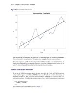
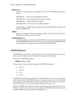
Figure 8.1 Autocorrelated Time Series
Note that when the series is above (or below) the OLS regression trend line, it tends to remain above
(below) the trend for several periods. This pattern is an example of positive autocorrelation.
Time series regression usually involves independent variables other than a time trend. However, the
simple time trend model is convenient for illustrating regression with autocorrelated errors, and the
series Y shown in Figure 8.1 is used in the following introductory examples.
Ordinary Least Squares Regression
To use the AUTOREG procedure, specify the input data set in the PROC AUTOREG statement
and specify the regression model in a MODEL statement. Specify the model by first naming the
dependent variable and then listing the regressors after an equal sign, as is done in other SAS
regression procedures. The following statements regress Y on TIME by using ordinary least squares:
proc autoreg data=a;
model y = time;
run;
The AUTOREG procedure output is shown in Figure 8.2.
Regression with Autocorrelated Errors ✦ 323
Figure 8.2 PROC AUTOREG Results for OLS Estimation
Autocorrelated Time Series
The AUTOREG Procedure
Dependent Variable y
Ordinary Least Squares Estimates
SSE 214.953429 DFE 34
MSE 6.32216 Root MSE 2.51439
SBC 173.659101 AIC 170.492063
MAE 2.01903356 AICC 170.855699
MAPE 12.5270666 HQC 171.597444
Durbin-Watson 0.4752 Regress R-Square 0.8200
Total R-Square 0.8200
Parameter Estimates
Standard Approx

Variable DF Estimate Error t Value Pr > |t|
Intercept 1 8.2308 0.8559 9.62 <.0001
time 1 0.5021 0.0403 12.45 <.0001
The output first shows statistics for the model residuals. The model root mean square error (Root
MSE) is 2.51, and the model
R
2
is 0.82. Notice that two
R
2
statistics are shown, one for the
regression model (Reg Rsq) and one for the full model (Total Rsq) that includes the autoregressive
error process, if any. In this case, an autoregressive error model is not used, so the two
R
2
statistics
are the same.
Other statistics shown are the sum of square errors (SSE), mean square error (MSE), mean absolute
error (MAE), mean absolute percentage error (MAPE), error degrees of freedom (DFE, the number
of observations minus the number of parameters), the information criteria SBC, HQC, AIC, and
AICC, and the Durbin-Watson statistic. (Durbin-Watson statistics, MAE, MAPE, SBC, HQC, AIC,
and AICC are discussed in the section “Goodness-of-fit Measures and Information Criteria” on
page 381 later in this chapter.)
The output then shows a table of regression coefficients, with standard errors and t tests. The
estimated model is
y
t
D 8:23 C 0:502t C 
t
Est: Var.

t
/ D 6:32
The OLS parameter estimates are reasonably close to the true values, but the estimated error variance,
6.32, is much larger than the true value, 4.
324 ✦ Chapter 8: The AUTOREG Procedure
Autoregressive Error Model
The following statements regress Y on TIME with the errors assumed to follow a second-order
autoregressive process. The order of the autoregressive model is specified by the NLAG=2 option.
The Yule-Walker estimation method is used by default. The example uses the METHOD=ML option
to specify the exact maximum likelihood method instead.
proc autoreg data=a;
model y = time / nlag=2 method=ml;
run;
The first part of the results is shown in Figure 8.3. The initial OLS results are produced first, followed
by estimates of the autocorrelations computed from the OLS residuals. The autocorrelations are also
displayed graphically.
Figure 8.3 Preliminary Estimate for AR(2) Error Model
Autocorrelated Time Series
The AUTOREG Procedure
Dependent Variable y
Ordinary Least Squares Estimates
SSE 214.953429 DFE 34
MSE 6.32216 Root MSE 2.51439
SBC 173.659101 AIC 170.492063
MAE 2.01903356 AICC 170.855699
MAPE 12.5270666 HQC 171.597444
Durbin-Watson 0.4752 Regress R-Square 0.8200
Total R-Square 0.8200
Parameter Estimates
Standard Approx

Variable DF Estimate Error t Value Pr > |t|
Intercept 1 8.2308 0.8559 9.62 <.0001
time 1 0.5021 0.0403 12.45 <.0001
Estimates of Autocorrelations
Lag Covariance Correlation -1 9 8 7 6 5 4 3 2 1 0 1 2 3 4 5 6 7 8 9 1
0 5.9709 1.000000 | |
********************
|
1 4.5169 0.756485 | |
***************
|
2 2.0241 0.338995 | |
*******
|
Preliminary MSE 1.7943
The maximum likelihood estimates are shown in Figure 8.4. Figure 8.4 also shows the preliminary
Yule-Walker estimates used as starting values for the iterative computation of the maximum likelihood
estimates.
Regression with Autocorrelated Errors ✦ 325
Figure 8.4 Maximum Likelihood Estimates of AR(2) Error Model
Estimates of Autoregressive Parameters
Standard
Lag Coefficient Error t Value
1 -1.169057 0.148172 -7.89
2 0.545379 0.148172 3.68
Algorithm converged.
Maximum Likelihood Estimates
SSE 54.7493022 DFE 32
MSE 1.71092 Root MSE 1.30802
SBC 133.476508 AIC 127.142432

MAE 0.98307236 AICC 128.432755
MAPE 6.45517689 HQC 129.353194
Durbin-Watson 2.2761 Regress R-Square 0.7280
Total R-Square 0.9542
Parameter Estimates
Standard Approx
Variable DF Estimate Error t Value Pr > |t|
Intercept 1 7.8833 1.1693 6.74 <.0001
time 1 0.5096 0.0551 9.25 <.0001
AR1 1 -1.2464 0.1385 -9.00 <.0001
AR2 1 0.6283 0.1366 4.60 <.0001
Autoregressive parameters assumed given
Standard Approx
Variable DF Estimate Error t Value Pr > |t|
Intercept 1 7.8833 1.1678 6.75 <.0001
time 1 0.5096 0.0551 9.26 <.0001
The diagnostic statistics and parameter estimates tables in Figure 8.4 have the same form as in
the OLS output, but the values shown are for the autoregressive error model. The MSE for the
autoregressive model is 1.71, which is much smaller than the true value of 4. In small samples, the
autoregressive error model tends to underestimate 
2
, while the OLS MSE overestimates 
2
.
Notice that the total
R
2
statistic computed from the autoregressive model residuals is 0.954, reflecting
the improved fit from the use of past residuals to help predict the next Y value. The Reg Rsq
value 0.728 is the

R
2
statistic for a regression of transformed variables adjusted for the estimated
autocorrelation. (This is not the
R
2
for the estimated trend line. For details, see the section
“Goodness-of-fit Measures and Information Criteria” on page 381 later in this chapter.)
326 ✦ Chapter 8: The AUTOREG Procedure
The parameter estimates table shows the ML estimates of the regression coefficients and includes
two additional rows for the estimates of the autoregressive parameters, labeled AR(1) and AR(2).
The estimated model is
y
t
D 7:88 C 0:5096t C 
t

t
D 1:25
t1
 0:628
t2
C 
t
Est: Var.
t
/ D 1:71
Note that the signs of the autoregressive parameters shown in this equation for 
t
are the reverse of

the estimates shown in the AUTOREG procedure output. Figure 8.4 also shows the estimates of the
regression coefficients with the standard errors recomputed on the assumption that the autoregressive
parameter estimates equal the true values.
Predicted Values and Residuals
The AUTOREG procedure can produce two kinds of predicted values and corresponding residuals
and confidence limits. The first kind of predicted value is obtained from only the structural part of
the model,
x
0
t
b
. This is an estimate of the unconditional mean of the response variable at time t. For
the time trend model, these predicted values trace the estimated trend. The second kind of predicted
value includes both the structural part of the model and the predicted values of the autoregressive
error process. The full model (conditional) predictions are used to forecast future values.
Use the OUTPUT statement to store predicted values and residuals in a SAS data set and to output
other values such as confidence limits and variance estimates. The P= option specifies an output
variable to contain the full model predicted values. The PM= option names an output variable for the
predicted mean. The R= and RM= options specify output variables for the corresponding residuals,
computed as the actual value minus the predicted value.
The following statements store both kinds of predicted values in the output data set. (The printed
output is the same as previously shown in Figure 8.3 and Figure 8.4.)
proc autoreg data=a;
model y = time / nlag=2 method=ml;
output out=p p=yhat pm=trendhat;
run;
The following statements plot the predicted values from the regression trend line and from the full
model together with the actual values:
title 'Predictions for Autocorrelation Model';
proc sgplot data=p;

scatter x=time y=y / markerattrs=(color=blue);
series x=time y=yhat / lineattrs=(color=blue);
series x=time y=trendhat / lineattrs=(color=black);
run;
The plot of predicted values is shown in Figure 8.5.
Forecasting Autoregressive Error Models ✦ 327
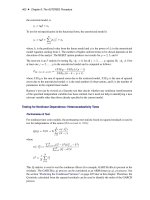
Figure 8.5 PROC AUTOREG Predictions
In Figure 8.5 the straight line is the autocorrelation corrected regression line, traced out by the
structural predicted values TRENDHAT. The jagged line traces the full model prediction values.
The actual values are marked by asterisks. This plot graphically illustrates the improvement in fit
provided by the autoregressive error process for highly autocorrelated data.
Forecasting Autoregressive Error Models
To produce forecasts for future periods, include observations for the forecast periods in the input data
set. The forecast observations must provide values for the independent variables and have missing
values for the response variable.
For the time trend model, the only regressor is time. The following statements add observations for
time periods 37 through 46 to the data set A to produce an augmented data set B:
328 ✦ Chapter 8: The AUTOREG Procedure
data b;
y = .;
do time = 37 to 46; output; end;
run;
data b;
merge a b;
by time;
run;
To produce the forecast, use the augmented data set as input to PROC AUTOREG, and specify the
appropriate options in the OUTPUT statement. The following statements produce forecasts for the
time trend with autoregressive error model. The output data set includes all the variables in the input
data set, the forecast values (YHAT), the predicted trend (YTREND), and the upper (UCL) and lower

(LCL) 95% confidence limits.
proc autoreg data=b;
model y = time / nlag=2 method=ml;
output out=p p=yhat pm=ytrend
lcl=lcl ucl=ucl;
run;
The following statements plot the predicted values and confidence limits, and they also plot the trend
line for reference. The actual observations are shown for periods 16 through 36, and a reference line
is drawn at the start of the out-of-sample forecasts.
title 'Forecasting Autocorrelated Time Series';
proc sgplot data=p;
band x=time upper=ucl lower=lcl;
scatter x=time y=y;
series x=time y=yhat;
series x=time y=ytrend / lineattrs=(color=black);
run;
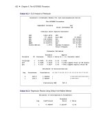
The plot is shown in Figure 8.6. Notice that the forecasts take into account the recent departures
from the trend but converge back to the trend line for longer forecast horizons.
Testing for Autocorrelation ✦ 329
Figure 8.6 PROC AUTOREG Forecasts
Testing for Autocorrelation
In the preceding section, it is assumed that the order of the autoregressive process is known. In
practice, you need to test for the presence of autocorrelation.
The Durbin-Watson test is a widely used method of testing for autocorrelation. The first-order Durbin-
Watson statistic is printed by default. This statistic can be used to test for first-order autocorrelation.
Use the DWPROB option to print the significance level (p-values) for the Durbin-Watson tests.
(Since the Durbin-Watson p-values are computationally expensive, they are not reported by default.)
You can use the DW= option to request higher-order Durbin-Watson statistics. Since the ordinary
Durbin-Watson statistic tests only for first-order autocorrelation, the Durbin-Watson statistics for
higher-order autocorrelation are called generalized Durbin-Watson statistics.

The following statements perform the Durbin-Watson test for autocorrelation in the OLS residuals
for orders 1 through 4. The DWPROB option prints the marginal significance levels (p-values) for
the Durbin-Watson statistics.
330 ✦ Chapter 8: The AUTOREG Procedure
/
*
Durbin-Watson test for autocorrelation
*
/
proc autoreg data=a;
model y = time / dw=4 dwprob;
run;
The AUTOREG procedure output is shown in Figure 8.7. In this case, the first-order Durbin-Watson
test is highly significant, with p < .0001 for the hypothesis of no first-order autocorrelation. Thus,
autocorrelation correction is needed.
Figure 8.7 Durbin-Watson Test Results for OLS Residuals
Forecasting Autocorrelated Time Series
The AUTOREG Procedure
Dependent Variable y
Ordinary Least Squares Estimates
SSE 214.953429 DFE 34
MSE 6.32216 Root MSE 2.51439
SBC 173.659101 AIC 170.492063
MAE 2.01903356 AICC 170.855699
MAPE 12.5270666 HQC 171.597444
Regress R-Square 0.8200
Total R-Square 0.8200
Durbin-Watson Statistics
Order DW Pr < DW Pr > DW
1 0.4752 <.0001 1.0000

2 1.2935 0.0137 0.9863
3 2.0694 0.6545 0.3455
4 2.5544 0.9818 0.0182
NOTE: Pr<DW is the p-value for testing positive autocorrelation, and Pr>DW is
the p-value for testing negative autocorrelation.
Parameter Estimates
Standard Approx
Variable DF Estimate Error t Value Pr > |t|
Intercept 1 8.2308 0.8559 9.62 <.0001
time 1 0.5021 0.0403 12.45 <.0001
Using the Durbin-Watson test, you can decide if autocorrelation correction is needed. However,
generalized Durbin-Watson tests should not be used to decide on the autoregressive order. The higher-
order tests assume the absence of lower-order autocorrelation. If the ordinary Durbin-Watson test
indicates no first-order autocorrelation, you can use the second-order test to check for second-order
autocorrelation. Once autocorrelation is detected, further tests at higher orders are not appropriate.
In Figure 8.7, since the first-order Durbin-Watson test is significant, the order 2, 3, and 4 tests can be
ignored.
Testing for Autocorrelation ✦ 331
When using Durbin-Watson tests to check for autocorrelation, you should specify an order at least
as large as the order of any potential seasonality, since seasonality produces autocorrelation at the
seasonal lag. For example, for quarterly data use DW=4, and for monthly data use DW=12.
Lagged Dependent Variables
The Durbin-Watson tests are not valid when the lagged dependent variable is used in the regression
model. In this case, the Durbin h test or Durbin t test can be used to test for first-order autocorrelation.
For the Durbin h test, specify the name of the lagged dependent variable in the LAGDEP= option.
For the Durbin t test, specify the LAGDEP option without giving the name of the lagged dependent
variable.
For example, the following statements add the variable YLAG to the data set A and regress Y on
YLAG instead of TIME:
data b;

set a;
ylag = lag1( y );
run;
proc autoreg data=b;
model y = ylag / lagdep=ylag;
run;
The results are shown in Figure 8.8. The Durbin h statistic 2.78 is significant with a p-value of
0.0027, indicating autocorrelation.
Figure 8.8 Durbin h Test with a Lagged Dependent Variable
Forecasting Autocorrelated Time Series
The AUTOREG Procedure
Dependent Variable y
Ordinary Least Squares Estimates
SSE 97.711226 DFE 33
MSE 2.96095 Root MSE 1.72074
SBC 142.369787 AIC 139.259091
MAE 1.29949385 AICC 139.634091
MAPE 8.1922836 HQC 140.332903
Regress R-Square 0.9109
Total R-Square 0.9109
Miscellaneous Statistics
Statistic Value Prob Label
Durbin h 2.7814 0.0027 Pr > h