SAS/ETS 9.22 User''''s Guide 75 pot

732 ✦ Chapter 13: The ESM Procedure
For example, PLOT=FORECASTS plots the forecasts for each series. The PLOT= option
produces printed output for these results by using the Output Delivery System (ODS).
PRINT=option | ( options )
specifies the printed output desired. By default, the ESM procedure produces no printed output.
The following printing options are available:
ESTIMATES prints the results of parameter estimation.
FORECASTS prints the forecasts.
PERFORMANCE prints the performance statistics for each forecast.
PERFORMANCESUMMARY prints the performance summary for each BY group.
PERFORMANCEOVERALL prints the performance summary for all of the BY groups.
STATISTICS prints the statistics of fit.
STATES prints the backcast, initial, and final states.
SUMMARY prints the summary statistics for the accumulated time series.
ALL
Same as PRINT=(ESTIMATES FORECASTS STATISTICS SUM-
MARY).
For example, PRINT=FORECASTS prints the forecasts, PRINT=(ESTIMATES FORE-
CASTS) prints the parameter estimates and the forecasts, and PRINT=ALL prints all of
the output.
PRINTDETAILS
specifies that output requested with the PRINT= option be printed in greater detail.
SEASONALITY=number
specifies the length of the seasonal cycle. For example, SEASONALITY=3 means that every
group of three observations forms a seasonal cycle. The SEASONALITY= option is applicable
only for seasonal forecasting models. By default, the length of the seasonal cycle is one (no
seasonality) or the length implied by the INTERVAL= option specified in the ID statement.
For example, INTERVAL=MONTH implies that the length of the seasonal cycle is twelve.
SORTNAMES
specifies that the variables specified in the FORECAST statements are processed in sorted
order.

STARTSUM=n
specifies the starting forecast lead (or horizon) for which to begin summation of the forecasts
specified by the LEAD= option. The STARTSUM= value must be less than the LEAD= value.
The default is STARTSUM=1; that is, the sum from the one-step ahead forecast (which is the
first forecast in the forecast horizon) to the multistep forecast specified by the LEAD= option.
The prediction standard errors of the summation of forecasts take into account the correlation
between the multistep forecasts. The section “Forecast Summation” on page 742 describes the
STARTSUM= option in more detail.
BY Statement ✦ 733
BY Statement
BY variables ;
A BY statement can be used with PROC ESM to obtain separate dummy variable definitions for
groups of observations defined by the BY variables.
When a BY statement appears, the procedure expects the input data set to be sorted in order of the
BY variables.
If your input data set is not sorted in ascending order, use one of the following alternatives:
 Sort the data by using the SORT procedure with a similar BY statement.

Specify the option NOTSORTED or DESCENDING in the BY statement for the ESM proce-
dure. The NOTSORTED option does not mean that the data are unsorted but rather that the
data are arranged in groups (according to values of the BY variables) and that these groups are
not necessarily in alphabetical or increasing numeric order.
 Create an index on the BY variables by using the DATASETS procedure.
For more information about the BY statement, see SAS Language Reference: Concepts. For more
information about the DATASETS procedure, see the discussion in the Base SAS Procedures Guide.
FORECAST Statement
FORECAST variable-list / options ;
The FORECAST statement lists the numeric variables in the DATA= data set whose accumulated
values represent time series to be modeled and forecast. The options specify which forecast model is
to be used.

A data set variable can be specified in only one FORECAST statement. Any number of FORECAST
statements can be used. The following options can be used with the FORECAST statement.
ACCUMULATE=option
specifies how the data set observations are accumulated within each time period for the
variables listed in the FORECAST statement. If the ACCUMULATE= option is not specified
in the FORECAST statement, accumulation is determined by the ACCUMULATE= option
of the ID statement. Use the ACCUMULATE= option with multiple FORECAST statements
when you want different accumulation specifications for different variables. See the ID
statement ACCUMULATE= option for more details.
ALPHA=number
specifies the significance level to use in computing the confidence limits of the forecast. The
ALPHA= value must be between 0 and 1. The default is ALPHA=0.05, which produces 95%
confidence intervals.
734 ✦ Chapter 13: The ESM Procedure
MEDIAN
specifies that the median forecast values are to be estimated. Forecasts can be based on the
mean or median. By default, the mean value is provided. If no transformation is applied to
the time series by using the TRANSFORM= option, the mean and median forecast values are
identical.
MODEL=model-name
specifies the forecasting model to be used to forecast the time series. The default is
MODEL=SIMPLE, which performs simple exponential smoothing. The following forecasting
models are provided:
NONE no forecast
SIMPLE simple (single) exponential smoothing. This is the default.
DOUBLE double (Brown) exponential smoothing
LINEAR linear (Holt) exponential smoothing
DAMPTREND damped trend exponential smoothing
ADDSEASONAL|SEASONAL additive seasonal exponential smoothing
MULTSEASONAL multiplicative seasonal exponential smoothing

WINTERS Winters multiplicative method
ADDWINTERS Winters additive method
When the option MODEL=NONE is specified, the time series is appended with missing values
in the OUT= data set. This option is useful when the results stored in the OUT= data set
are used in a subsequent analysis where forecasts of the independent variables are needed to
forecast the dependent variable.
NBACKCAST=n
specifies the number of observations used to initialize the backcast states. The default is the
entire series.
REPLACEBACK
specifies that actual values excluded by the BACK= option are replaced with one-step-ahead
forecasts in the OUT= data set.
REPLACEMISSING
specifies that embedded missing values are replaced with one-step-ahead forecasts in the
OUT= data set.
SETMISSING=option | number
specifies how missing values (either input or accumulated) are assigned in the accumulated
time series for variables listed in the FORECAST statement. If the SETMISSING= option is
not specified in the FORECAST statement, missing values are set based on the SETMISSING=
option of the ID statement. See the ID statement SETMISSING= option for more details.
TRANSFORM=option
specifies the time series transformation to be applied to the input or accumulated time series.
The following transformations are provided:
ID Statement ✦ 735
NONE no transformation. This is the default.
LOG logarithmic transformation
SQRT square-root transformation
LOGISTIC logistic transformation
BOXCOX(n)
Box-Cox transformation with parameter number where number is between

–5 and 5
When the TRANSFORM= option is specified, the time series must be strictly positive. After
the time series is transformed, the model parameters are estimated by using the transformed
series. The forecasts of the transformed series are then computed, and finally the transformed
series forecasts are inverse transformed. The inverse transform produces either mean or
median forecasts depending on whether the MEDIAN option is specified. The sections
“Transformations” on page 741 and “Inverse Transformations” on page 742 describe this in
more detail.
USE=option
specifies which forecast values are appended to the actual values in the OUT= and OUTSUM=
data sets. The following USE= options are provided:
PREDICT
The predicted values are appended to the actual values. This option is the
default.
LOWER The lower confidence limit values are appended to the actual values.
UPPER The upper confidence limit values are appended to the actual values.
Thus, the USE= option enables the OUT= and OUTSUM= data sets to be used for worst-case,
best-case, average-case, and median-case decisions.
ZEROMISS=option
specifies how beginning or ending zero values (either input or accumulated) are interpreted
in the accumulated time series for variables listed in the FORECAST statement. If the
ZEROMISS= option is not specified in the FORECAST statement, beginning or ending zero
values are set to missing values based on the ZEROMISS= option of the ID statement. See the
ID statement ZEROMISS= option for more details.
ID Statement
ID variable INTERVAL= interval < options > ;
The ID statement names a numeric variable that identifies observations in the input and output data
sets. The ID variable’s values are assumed to be SAS date or datetime values. In addition, the ID
statement specifies the (desired) frequency associated with the time series. The ID statement options
also specify how the observations are accumulated and how the time ID values are aligned to form

the time series to be forecast. The information specified affects all variables specified in subsequent
FORECAST statements. If the ID statement is specified, the INTERVAL= option must be specified.
736 ✦ Chapter 13: The ESM Procedure
If an ID statement is not specified, the observation number, with respect to the BY group, is used as
the time ID. The following options can be used with the ID statement.
ACCUMULATE=option
specifies how the data set observations are accumulated within each time period. The frequency
(width of each time interval) is specified by the INTERVAL= option. The ID variable contains
the time ID values. Each time ID variable value corresponds to a specific time period. The
accumulated values form the time series, which is used in subsequent model fitting and
forecasting.
The ACCUMULATE= option is particularly useful when there are gaps in the input data or
when there are multiple input observations that coincide with a particular time period (for
example, transactional data). The EXPAND procedure offers additional frequency conversions
and transformations that can also be useful in creating a time series.
The following options determine how the observations are accumulated within each time
period based on the ID variable and the frequency specified by the INTERVAL= option:
NONE
No accumulation occurs; the ID variable values must be equally
spaced with respect to the frequency. This is the default option.
TOTAL
Observations are accumulated based on the total sum of their val-
ues.
AVERAGE | AVG
Observations are accumulated based on the average of their values.
MINIMUM | MIN
Observations are accumulated based on the minimum of their
values.
MEDIAN | MED
Observations are accumulated based on the median of their values.

MAXIMUM | MAX
Observations are accumulated based on the maximum of their
values.
N
Observations are accumulated based on the number of nonmissing
observations.
NMISS
Observations are accumulated based on the number of missing
observations.
NOBS
Observations are accumulated based on the number of observa-
tions.
FIRST Observations are accumulated based on the first of their values.
LAST Observations are accumulated based on the last of their values.
STDDEV | STD
Observations are accumulated based on the standard deviation of
their values.
CSS
Observations are accumulated based on the corrected sum of
squares of their values.
USS
Observations are accumulated based on the uncorrected sum of
squares of their values.
ID Statement ✦ 737
If the ACCUMULATE= option is specified, the SETMISSING= option is useful for specifying
how accumulated missing values are treated. If missing values should be interpreted as zero,
then SETMISSING=0 should be used. The section “Accumulation” on page 739 describes
accumulation in greater detail.
ALIGN=option
controls the alignment of SAS dates used to identify output observations. The ALIGN= option

accepts the following values: BEGINNING | BEG | B, MIDDLE | MID | M, and ENDING |
END | E. BEGINNING is the default.
END=date | datetime
specifies a SAS date or datetime literal value that represents the end of the data. If the last time
ID variable value is less than the END= value, the series is extended with missing values. If the
last time ID variable value is greater than the END= value, the series is truncated. For example,
END=‘1jan2008’D
specifies that data for time periods after the first of January 2008 not be
used. The option
END=“&sysdate”D
uses the automatic macro variable SYSDATE to extend
or truncate the series to the current date. This option and the START= option can be used to
ensure that data associated with each BY group contains the same number of observations.
FORMAT=format
specifies the SAS format for the time ID values. If the FORMAT= option is not specified, the
default format is implied from the INTERVAL= option.
INTERVAL=interval
specifies the frequency of the input time series or for the time series to be accumulated from
the input data. For example, if the input data set consists of quarterly observations, then
INTERVAL=QTR should be used. If the SEASONALITY= option is not specified, the length
of the seasonal cycle is implied by the INTERVAL= option. For example, INTERVAL=QTR
implies a seasonal cycle of length 4. If the ACCUMULATE= option is also specified, the
INTERVAL= option determines the time periods for the accumulation of observations.
The basic intervals are YEAR, SEMIYEAR, QTR, MONTH, SEMIMONTH, TENDAY,
WEEK, WEEKDAY, DAY, HOUR, MINUTE, SECOND. See Chapter 4, “Date Intervals,
Formats, and Functions,” for more information about the intervals that can be specified.
NOTSORTED
specifies that the time ID values are not in sorted order. The ESM procedure sorts the data
with respect to the time ID prior to analysis.
SETMISSING=option | number

specifies how missing values (either input or accumulated) are assigned in the accumulated
time series. If a number is specified, missing values are set to that number. If a missing value
on the input data set indicates an unknown value, the SETMISSING= option should not be
used. If a missing value indicates no value, SETMISSING=0 should be used. You typically use
SETMISSING=0 for transactional data, because no recorded data usually implies no activity.
The following options can also be used to determine how missing values are assigned:
MISSING Missing values are set to missing. This is the default option.
AVERAGE | AVG Missing values are set to the accumulated average value.
738 ✦ Chapter 13: The ESM Procedure
MINIMUM | MIN Missing values are set to the accumulated minimum value.
MEDIAN | MED Missing values are set to the accumulated median value.
MAXIMUM | MAX Missing values are set to the accumulated maximum value.
FIRST Missing values are set to the accumulated first nonmissing value.
LAST Missing values are set to the accumulated last nonmissing value.
PREVIOUS | PREV
Missing values are set to the previous accumulated nonmissing
value. Missing values at the beginning of the accumulated series
remain missing.
NEXT
Missing values are set to the next accumulated nonmissing value.
Missing values at the end of the accumulated series remain missing.
If SETMISSING=MISSING is specified, the missing observations are replaced with predicted
values computed from the exponential smoothing model.
START=date | datetime
specifies a SAS date or datetime literal value that represents the beginning of the data. If
the first time ID variable value is greater than the START= value, the series is prefixed with
missing values. If the first time ID variable value is less than the START= value, the series is
truncated. This option and the END= option can be used to ensure that data associated with
each BY group contains the same number of observations.
ZEROMISS=option

specifies how beginning and/or ending zero values (either input or accumulated) are interpreted
in the accumulated time series. The following values can be specified for the ZEROMISS=
option:
NONE Beginning and/or ending zeros are unchanged. This is the default.
LEFT Beginning zeros are set to missing.
RIGHT Ending zeros are set to missing.
BOTH Both beginning and ending zeros are set to missing.
If the accumulated series is all missing and/or zero the series is not changed.
Details: ESM Procedure
The ESM procedure can be used to forecast time series data as well as transactional data. If the data
is transactional, then the procedure must first accumulate the data into a time series before it can be
forecast. The procedure uses the following sequential steps to produce forecasts, with the options
that control the step listed to the right:
Accumulation ✦ 739
Table 13.2 ESM Processing Steps and Control Options
Step Operation Option Statement
1 accumulation ACCUMULATE= ID
2 missing value interpretation SETMISSING= ID, FORECAST
3 transformations TRANSFORM= FORECAST
4 parameter estimation MODEL= FORECAST
5 forecasting MODEL=, LEAD= FORECAST, PROC ESM
6 inverse transformation TRANSFORM, MEDIAN FORECAST
7 summation of forecasts LEAD=, STARTSUM= PROC ESM
Each of the steps shown in Table 13.2 is described in the following sections.
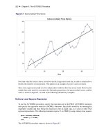
Accumulation
If the ACCUMULATE= option is specified in the ID statement, data set observations are accumulated
within each time period. The frequency (width of each time interval) is specified by the INTERVAL=
option, and the ID variable contains the time ID values. Each time ID value corresponds to a specific
time period. Accumulation is particularly useful when the input data set contains transactional data,
whose observations are not spaced with respect to any particular time interval. The accumulated

values form the time series that is used in subsequent analyses by the ESM procedure.
For example, suppose a data set contains the following observations:
19MAR1999 10
19MAR1999 30
11MAY1999 50
12MAY1999 20
23MAY1999 20
If the INTERVAL=MONTH option is specified on the ID statement, all of the preceding observations
fall within three time periods: March 1999, April 1999, and May 1999. The observations are
accumulated within each time period as follows.
If the ACCUMULATE=NONE option is specified, an error is generated because the ID variable
values are not equally spaced with respect to the specified frequency (MONTH).
If the ACCUMULATE=TOTAL option is specified, the resulting time series is:
O1MAR1999 40
O1APR1999 .
O1MAY1999 90
If the ACCUMULATE=AVERAGE option is specified, the resulting time series is:
740 ✦ Chapter 13: The ESM Procedure
O1MAR1999 20
O1APR1999 .
O1MAY1999 30
If the ACCUMULATE=MINIMUM option is specified, the resulting time series is:
O1MAR1999 10
O1APR1999 .
O1MAY1999 20
If the ACCUMULATE=MEDIAN option is specified, the resulting time series is:
O1MAR1999 20
01APR1999 .
O1MAY1999 20
If the ACCUMULATE=MAXIMUM option is specified, the resulting time series is:

O1MAR1999 30
O1APR1999 .
O1MAY1999 50
If the ACCUMULATE=FIRST option is specified, the resulting time series is:
O1MAR1999 10
O1APR1999 .
O1MAY1999 50
If the ACCUMULATE=LAST option is specified, the resulting time series is:
O1MAR1999 30
O1APR1999 .
O1MAY1999 20
If the ACCUMULATE=STDDEV option is specified, the resulting time series is:
O1MAR1999 14.14
O1APR1999 .
O1MAY1999 17.32
As can be seen from the preceding examples, even though the data set observations contained no
missing values, the accumulated time series can have missing values.
Missing Value Interpretation ✦ 741
Missing Value Interpretation
Sometimes missing values should be interpreted as truly unknown values and retained as missing
values in the data set. The forecasting models used by the ESM procedure can effectively handle
missing values (see the section “Missing Value Modeling Issues” on page 741). However, sometimes
missing values are known, such as when missing values are created from accumulation and represent
no observed values for the variable. In this case, the value for the period should be interpreted as zero
(no values), and the SETMISSING=0 option should be used to cause PROC ESM to recode missing
values as zero. In other cases, missing values should be interpreted as global values, such as minimum
or maximum values of the accumulated series. The accumulated and missing-value-recoded time
series is used in subsequent analyses in PROC ESM.
Transformations
If the TRANSFORM= option is specified in the FORECAST statement, the time series is transformed

prior to model parameter estimation and forecasting. Only strictly positive series can be transformed.
An error is generated when the TRANSFORM= option is used with a nonpositive series. (See
Chapter 46, “Forecasting Process Details,” for more details about forecasting transformed time
series.)
Parameter Estimation
All the parameters (smoothing weights) associated with the exponential smoothing model used to
forecast the time series (as specified by the MODEL= option) are optimized based on the data,
with the default parameter restrictions imposed. If the TRANSFORM= option is specified, the
transformed time series data are used to estimate the model parameters.
The techniques used in the ESM procedure are identical to those used for exponential smoothing
models in the Time Series Forecasting System of SAS/ETS software. See Chapter 38, “Overview of
the Time Series Forecasting System,” for more information.
Missing Value Modeling Issues
The treatment of missing values varies with the forecasting model. Missing values after the start of
the series are replaced with one-step-ahead predicted values, and the predicted values are used in the
smoothing equations.
The treatment of missing values can also be specified with the SETMISSING= option, which changes
the missing values prior to modeling.