SAS/ETS 9.22 User''''s Guide 113 potx

1112 ✦ Chapter 18: The MODEL Procedure
Error Covariance Structure Specification
One of the key assumptions of regression is that the variance of the errors is constant across
observations. Correcting for heteroscedasticity improves the efficiency of the estimates.
Consider the following general form for models:
q.y
t
; x
t
; Â/ D "
t
"
t
D H
t
 
t
H
t
D
2
6
6
6
4
p
h
t;1
0 : : : 0
0
p

h
t;2
: : : 0
:
:
:
0 0 : : :
p
h
t;g
3
7
7
7
5
h
t
D g.y
t
; x
t
; /
where 
t
 N.0; †/.
For models that are homoscedastic,
h
t
D 1
If you have a model that is heteroscedastic with known form, you can improve the efficiency of the

estimates by performing a weighted regression. The weight variable, using this notation, would be
1=
p
h
t
.
If the errors for a model are heteroscedastic and the functional form of the variance is known, the
model for the variance can be estimated along with the regression function.
To specify a functional form for the variance, assign the function to an H.var variable where var is
the equation variable. For example, if you want to estimate the scale parameter for the variance of a
simple regression model
y D a  x C b
you can specify
proc model data=s;
y = a
*
x + b;
h.y = sigma
**
2;
fit y;
Consider the same model with the following functional form for the variance:
h
t
D 
2
 x
2˛
This would be written as
Error Covariance Structure Specification ✦ 1113

proc model data=s;
y = a
*
x + b;
h.y = sigma
**
2
*
x
**
(2
*
alpha);
fit y;
There are three ways to model the variance in the MODEL procedure: feasible generalized least
squares, generalized method of moments, and full information maximum likelihood.
Feasible GLS
A simple approach to estimating a variance function is to estimate the mean parameters
Â
by using
some auxiliary method, such as OLS, and then use the residuals of that estimation to estimate the
parameters

of the variance function. This scheme is called feasible GLS. It is possible to use
the residuals from an auxiliary method for the purpose of estimating

because in many cases the
residuals consistently estimate the error terms.
For all estimation methods except GMM and FIML, using the H.var syntax specifies that feasible
GLS is used in the estimation. For feasible GLS, the mean function is estimated by the usual method.

The variance function is then estimated using pseudo-likelihood (PL) function of the generated
residuals. The objective function for the PL estimation is
p
n
.; Â/ D
n
X
iD1

.y
i
 f .x
i
;
O
ˇ//
2

2
h.z
i
; Â/
C logŒ
2
h.z
i
; Â/
!
Once the variance function has been estimated, the mean function is reestimated by using the variance
function as weights. If an S-iterated method is selected, this process is repeated until convergence

(iterated feasible GLS).
Note that feasible GLS does not yield consistent estimates when one of the following is true:
 The variance is unbounded.
 There is too much serial dependence in the errors (the dependence does not fade with time).
 There is a combination of serial dependence and lag dependent variables.
The first two cases are unusual, but the third is much more common. Whether iterated feasible
GLS avoids consistency problems with the last case is an unanswered research question. For more
information see Davidson and MacKinnon (1993, pp. 298–301) or Gallant (1987, pp. 124–125) and
Amemiya (1985, pp. 202–203).
One limitation is that parameters cannot be shared between the mean equation and the variance
equation. This implies that certain GARCH models, cross-equation restrictions of parameters, or
testing of combinations of parameters in the mean and variance component are not allowed.
1114 ✦ Chapter 18: The MODEL Procedure
Generalized Method of Moments
In GMM, normally the first moment of the mean function is used in the objective function.
q.y
t
; x
t
; Â/ D 
t
E.
t
/ D 0
To add the second moment conditions to the estimation, add the equation
E."
t
 "
t
 h

t
/ D 0
to the model. For example, if you want to estimate  for linear example above, you can write
proc model data=s;
y = a
*
x + b;
eq.two = resid.y
**
2 - sigma
**
2;
fit y two/ gmm;
instruments x;
run;
This is a popular way to estimate a continuous-time interest rate processes (see Chan et al. 1992).
The H.var syntax automatically generates this system of equations.
To further take advantage of the information obtained about the variance, the moment equations can
be modified to
E."
t
=
p
h
t
/ D 0
E."
t
 "
t

 h
t
/ D 0
For the above example, this can be written as
proc model data=s;
y = a
*
x + b;
eq.two = resid.y
**
2 - sigma
**
2;
resid.y = resid.y / sigma;
fit y two/ gmm;
instruments x;
run;
Note that, if the error model is misspecified in this form of the GMM model, the parameter estimates
might be inconsistent.
Error Covariance Structure Specification ✦ 1115
Full Information Maximum Likelihood
For FIML estimation of variance functions, the concentrated likelihood below is used as the objective
function. That is, the mean function is coupled with the variance function and the system is solved
simultaneously.
l
n
./ D
ng
2
.1 C ln.2// 

n
X
tD1
ln
Â
ˇ
ˇ
ˇ
ˇ
@q.y
t
; x
t
; Â/
@y
t
ˇ
ˇ
ˇ
ˇ
Ã
C
1
2
n
X
tD1
g
X
iD1


ln.h
t;i
/ C q
i
.y
t
; x
t
; Â/
2
=h
t;i

where g is the number of equations in the system.
The HESSIAN=GLS option is not available for FIML estimation that involves variance functions.
The matrix used when HESSIAN=CROSS is specified is a crossproducts matrix that has been
enhanced by the dual quasi-Newton approximation.
Examples
You can specify a GARCH(1,1) model as follows:
proc model data=modloc.usd_jpy;
/
*
Mean model
*
/
jpyret = intercept ;
/
*
Variance model

*
/
h.jpyret = arch0
+ arch1
*
xlag( resid.jpyret
**
2, mse.jpyret )
+ garch1
*
xlag(h.jpyret, mse.jpyret) ;
bounds arch0 arch1 garch1 >= 0;
fit jpyret / method=marquardt fiml;
run;
Note that the BOUNDS statement is used to ensure that the parameters are positive, a requirement
for GARCH models.
EGARCH models are used because there are no restrictions on the parameters. You can specify a
EGARCH(1,1) model as follows:
proc model data=sasuser.usd_dem ;
/
*
Mean model
*
/
demret = intercept ;
1116 ✦ Chapter 18: The MODEL Procedure
/
*
Variance model
*

/
if ( _OBS_ =1 ) then
h.demret = exp( earch0 + egarch1
*
log(mse.demret) );
else
h.demret = exp( earch0 + earch1
*
zlag( g)
+ egarch1
*
log(zlag(h.demret)));
g = - theta
*
nresid.demret + abs( nresid.demret ) - sqrt(2/3.1415);
fit demret / method=marquardt fiml maxiter=100 converge=1.0e-6;
run;
Ordinary Differential Equations
Ordinary differential equations (ODEs) are also called initial value problems because a time zero
value for each first-order differential equation is needed. The following is an example of a first-order
system of ODEs:
y
0
D 0:1y C2:5z
2
z
0
D z
y
0

D 0
z
0
D 1
Note that you must provide an initial value for each ODE.
As a reminder, any n-order differential equation can be modeled as a system of first-order differential
equations. For example, consider the differential equations
y
00
D by
0
C cy
y
0
D 0
y
0
0
D 1
which can be written as the system of differential equations
y
0
D z
z
0
D by
0
C cy
y
0

D 0
z
0
D 1
This differential system can be simulated as follows:
data t;
time=0; output;
time=1; output;
time=2; output;
Ordinary Differential Equations ✦ 1117
run;
proc model data=t ;
dependent y 0 z 1;
parm b -2 c -4;
dert.y = z;
dert.z = b
*
dert.y + c
*
y;
solve y z / dynamic solveprint;
run;
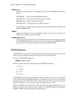
The preceding statements produce the output shown in Figure 18.44. These statements produce
additional output, which is not shown.
Figure 18.44 Simulation Results for Differential System
The MODEL Procedure
Simultaneous Simulation
Observation 1 Missing 2 CC -1.000000
Iterations 0
Solution Values

y z
0.000000 1.000000
Observation 2 Iterations 0 CC 0.000000 ERROR.y 0.000000
Solution Values
y z
0.2096398 2687053
Observation 3 Iterations 0 CC 9.464802 ERROR.y -0.234405
Solution Values
y z
0247649 1035929
The differential variables are distinguished by the derivative with respect to time (DERT.) prefix.
Once you define the DERT. variable, you can use it on the right-hand side of another equation.
The differential equations must be expressed in normal form; implicit differential equations are not
allowed, and other terms on the left-hand side are not allowed.
The TIME variable is the implied with respect to variable for all DERT. variables. The TIME variable
is also the only variable that must be in the input data set.
1118 ✦ Chapter 18: The MODEL Procedure
You can provide initial values for the differential equations in the data set, in the declaration statement
(as in the previous example), or in statements in the program. Using the previous example, you can
specify the initial values as
proc model data=t ;
dependent y z ;
parm b -2 c -4;
if ( time=0 ) then
do;
y=0;
z=1;
end;
else
do;

dert.y = z;
dert.z = b
*
dert.y + c
*
y;
end;
end;
solve y z / dynamic solveprint;
run;
If you do not provide an initial value, 0 is used.
DYNAMIC and STATIC Simulation
Note that, in the previous example, the DYNAMIC option is specified in the SOLVE statement. The
DYNAMIC and STATIC options work the same for differential equations as they do for dynamic
systems. In the differential equation case, the DYNAMIC option makes the initial value needed at
each observation the computed value from the previous iteration. For a static simulation, the data
set must contain values for the integrated variables. For example, if DERT.Y and DERT.Z are the
differential variables, you must include Y and Z in the input data set in order to do a static simulation
of the model.
If the simulation is dynamic, the initial values for the differential equations are obtained from the
data set, if they are available. If the variable is not in the data set, you can specify the initial value in
a declaration statement. If you do not specify an initial value, the value of 0.0 is used.
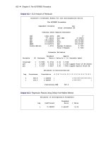
A dynamic solution is obtained by solving one initial value problem for all the data. A graph of a
simple dynamic simulation is shown in Figure 18.45. If the time variable for the current observation
is less than the time variable for the previous observation, the integration is restarted from this point.
This allows for multiple samples in one data file.
Ordinary Differential Equations ✦ 1119
Figure 18.45 Dynamic Solution
In a static solution, n–1 initial value problems are solved using the first n–1 data values as initial
values. The equations are integrated using the

i
th data value as an initial value to the i+1 data value.
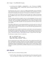
Figure 18.46 displays a static simulation of noisy data from a simple differential equation. The static
solution does not propagate errors in initial values as the dynamic solution does.
1120 ✦ Chapter 18: The MODEL Procedure
Figure 18.46 Static Solution
For estimation, the DYNAMIC and STATIC options in the FIT statement perform the same functions
as they do in the SOLVE statement. Components of differential systems that have missing values
or are not in the data set are simulated dynamically. For example, often in multiple compartment
kinetic models, only one compartment is monitored. The differential equations that describe the
unmonitored compartments are simulated dynamically.
For estimation, it is important to have accurate initial values for ODEs that are not in the data set.
If an accurate initial value is not known, the initial value can be made an unknown parameter and
estimated. This allows for errors in the initial values but increases the number of parameters to
estimate by the number of equations.
Estimation of Differential Equations
Consider the kinetic model for the accumulation of mercury (Hg) in mosquito fish (Matis, Miller,
and Allen 1991, p. 177). The model for this process is the one-compartment constant infusion model
shown in Figure 18.47.
Ordinary Differential Equations ✦ 1121
Figure 18.47 One-Compartment Constant Infusion Model
The differential equation that models this process is
dconc
dt
D k
u
 k
e
conc
conc

0
D 0
The analytical solution to the model is
conc D .k
u
=k
e
/.1  exp.k
e
t//
The data for the model are
data fish;
input day conc;
datalines;
0.0 0.0
1.0 0.15
2.0 0.2
3.0 0.26
4.0 0.32
6.0 0.33
;
To fit this model in differential form, use the following statements:
proc model data=fish;
parm ku ke;
dert.conc = ku - ke
*
conc;
fit conc / time=day;
run;
The results from this estimation are shown in Figure 18.48.