Six Sigma Fast Track Course
Bạn đang xem bản rút gọn của tài liệu. Xem và tải ngay bản đầy đủ của tài liệu tại đây (2.6 MB, 422 trang )
SIX SIGMA
FAST TRACK
COURSE
MAY 2008
Six Sigma Explained
Six Sigma is the popular name of a management system that uses data and systematic
approaches to continually improve the quality of business processes and consistently achieve
performance excellence. Simply stated, Six Sigma is a way for you to do things better,
faster, and for less cost.
The term "Six Sigma" was originally coined by General Electric and literally refers to a
statistical condition is which a process achieves a failure rate of less than 6 standard
deviations (the symbol for standard deviation is the Greek litter sigma), or 3.4 parts per
million. In this regard, achieving Six Sigma performance ideally means reducing undesirable
issues to a rate of less than 3.4 per million transactions. In reality however, few business
processes require true six sigma error levels and the term "Six Sigma" has adopted a more
general definition of "continually working toward making business processes as efficient as
possible."
Although Six Sigma is a relatively modern term, it borrows heavily from earlier management
philosophies such as Business Process Management, Total Quality Management, and others. If
you have any experience with these techniques, you will probably find much of Six Sigma
familiar.
The Five Major Areas Of Six Sigma
When Six Sigma is taught, it is generally broken down into five groups of related topics.
Since we are moving quickly, rather than covering each of the five areas in depth we will
instead provide a brief overview of each area and spend one page highlighting their purpose
and components. Let's begin by introducing each topic area:
Analytical Tools
Analytical tools are a collection of charts and graphs that help people understand and
communicate data. Some of these charts will be familiar to you while others, such as a
control chart, will probably be new. These tools are used when data must be organized,
displayed, or communicated to others in the Six Sigma process.
Decision-Making Tools
Decision-making tools are a collection of tools and techniques that help people make logical,
fact-based decisions based on data. These tools are used to prioritize options and make the
mathematically "best" decision based on the data available to the team. By making the best
decisions, a team has the highest possible probability of success.
Process Management
Process management is a step-by-step procedure that helps organizations understand what
they do, find better ways to do it, and ensure that improvements remain effective.
This technique is frequently used organization-wide to get a handle on what needs to be
improved and to ensure that improvement efforts are, and remain, effective.
DMAIC Problem Solving Process
DMAIC is a formal problem solving methodology for correcting an undesirable process
outcome performance and ensuring that corrective measures maintain acceptable
performance. When an organization encounters a problem, or when a business process is not
meeting its performance targets, the DMAIC process can be utilized to systematically reduce
or eliminate the problem.
Leadership / Strategic Planning
General leadership and strategic planning topics are often discussed as part of traditional Six
Sigma training. These include areas such as team dynamics, managing improvement
teams, and establishing clear linkages between Six Sigma efforts and organizational
objectives.
How We Will Discuss Six Sigma In This Course
Now that you have a general idea of the topics provided in a Six Sigma course, we'll spend
the remainder of this course two ways. First, we must quickly cover some simple concepts
and terminology that are used in Six Sigma. You need to learn some of the basics or it will
be difficult to understand DMAIC. Once that is finished we will dive right into practical Six
Sigma by walking, step-by-step, through the DMAIC problem solving process.
DMAIC is a good tool for teaching Six Sigma. As you learn each step in the DMAIC process,
you will see how many of the analytical and decision tools are applied, and you will view an
example DMAIC "story" to see exactly what the outcome of the structured problem solving
process looks like. Once you have a basic familiarity of the tools, techniques, and a
"structured process," you will have the minimum skills you need to begin applying DMAIC,
Process Management, or any other Six Sigma concept. Working through this process will also
demystify Six Sigma and show you why it works so well.
Now, before we jump into DMAIC, let's take a look at each of five Six Sigma topic areas
along with an index of links to each of their specific tools, techniques, and concepts.
Key Point
ets FasTrack
Summary 1 of 1:- -
What is the name of the management system that uses data and systematic approaches to continually improve
the quality of business processes and consistently achieve performance excellence?-
Answer: Six Sigma
What Are The Analytical Tools?
Below you will find a very brief overview of the major concepts introduced in the full
Electronic Training Solution (ets) Analytical Tools course. We will encounter many of these
tools and techniques as they are applied throughout his course. You are encouraged to skim
the list below and see if any of these concepts are unfamiliar to you. If so, please take a
moment to click on the item and read a short description of it.
Analytical Tools Are A Common Language For Data (Excerpted from the ets Analytical Tools
course)
Analytical Tools are a common language of charts and graphs that are used to
communicate information throughout your organization. Each chart and graph conveys
different information, but the purpose of each is to help you and others better
understand data.
During the course, you were introduced to some general concepts. Click on any of these
topics to return to the appropriate page in the course:
•
The Need For Source Blocks
•
Populations and Samples
•
Attribute Data vs. Variables Data
You also learned the purpose, application, and construction methods for the following
analytical tools. Click on any of these topics to return to the appropriate page in the course:
•
•
Checksheets or Electronic Spreadsheets
A Checksheet is a tool used to collect data.
•
Bar Charts
A Bar Chart is a "summary" graph used to compare the amount of an item with
other items.
•
Line Graphs
A Line Graph is a "trend" graph that displays process outputs or outcomes
sequenced by time or by occurrence.
•
Pie Charts
A Pie Chart is a "summary" graph that shows highlights data items' relationships to
their whole data set.
•
Pareto Charts
A Pareto Chart is a "summary" analysis tool that is used to rank data groups.
•
Cause and Effect Diagrams
A Cause and Effect Diagram is an analytical tool used to determine qualitative
relationships between a problem and the reasons or factors that are possibly
causing it.
•
Scatter Diagrams
The Scatter Diagram is an analytical tool that determines whether or not
a relationship exists between two linked or paired data sets.
•
Histograms
A Histogram is an analytical tool that displays how a group of data is distributed
from lowest to highest.
•
Control Charts
A Control Chart is a data analysis tool that helps you to monitor the stability of
a process output.
What are Source Blocks?
Maintaining Accountability
Just as you sign your name to a report, you should let others know that you are the source of
any analytical tool you create. Source blocks are small packages of information that are
attached to analytical tools so that readers know when the data was generated, where the
source data was taken from, and who they can contact if they have questions about the tool.
Many times analytical tools, such as charts and graphs, are reused or included in
presentations, marketing packages etc. Providing a source block ensures that even if your tool
is taken out of context, a reader can clearly determine the timeliness of your data and contact
the author if questions arise.
By requiring clear documentation of authors and dates, source blocks help maintain
accountability for analysis tools and encourage you to produce accurate work. They also
prevent others from misinterpreting your data or using outdated information.
The Typical Source Block
Source block formatting is the same for all data analysis tools. You should know what
information goes into a source block and the standard way they are constructed.
Each source block looks like a small table and should contain, at a minimum, the following
information:
When: This is the date when the data was collected, not when the tool was created or
revised. This value may be an exact date, a quarter, or even an event. If you are unsure
about what to put here, ask yourself what information that a reader would require to find the
exact information you used in creating your chart.
Where: This is the physical source of the data. The "Where" entry should provide enough
guidance so that any employee could locate the exact data used for this particular tool. Make
sure to specify exact locations, such as file paths or document numbers, if they are available.
Who: The "Who" entry lists all employees that created the tool. It is provided as a
reference so that coworkers may identify the authors of the tool in case they have questions,
corrections, or additions.
Figures 1 and 2 show example source blocks. Note the level of detail provided in each section
of the source block and the variation of the two styles. Locating data in a small company is
dramatically different compared to a multinational conglomerate. Make sure you provide
enough information for your organization.
Data Source Information
When: First Quarter, 2003 YTD
Where: Doc #11354-1 Human Resource Funding, P
19-27
Who: K. Abrahams x3386, C. Fenwick x1914
Figure 1: A Typical Source Block from a Large Organization
Data Source Information
When: October 3, 2003
Where: Accountant Report (From J. Peterson)
Who: Karen in Human Resources
Figure 2: A Typical Source Block from a Small Organization
Source blocks should be attached to every data management tool you produce. In fact, it is a
good practice to attach the source block prior to completing the tool to ensure your chart will
be accurately represented if someone pulls your chart off the printer or your desk while you
are at lunch.
Source blocks may be placed in any convenient location on your tool, but generally they are
kept in the lower right hand corner for consistency.
Sample vs. Population
What is the difference between a Sample and a Population?
You can collect information from ALL of the relevant things (every employee) or you can
sample a smaller sub-group of relevant things and use their results to represent the entire
group (20% of the employees).
When you collect data from everything in your relevant data set, this is called a "population"
of data. Populations are denoted by a capital "N." For example, if you have 450 employees
and you asked each one of them which flavor of ice cream they prefer, you have conducted a
population analysis where N = 450. Gathering population data is also called performing a
"census" of your data.
When you collect data from a representative portion of your entire relevant data set, this is
called a "sample" of data. Samples are denoted by a lowercase "n." If you instead only asked
100 of your 450 employees which ice cream flavor they prefer, you would have conducted a
sample analysis where n = 100. Gathering population data is also called performing a
"sample" of your data.
What makes data "relevant?"
If you are performing a study of employee satisfaction in your organization, your population
would include every single employee. This makes sense, since every employee has a relevant
stake in the company's overall satisfaction.
Consider, however, an employee satisfaction study of only your Human Resources
department. In this case, only HR employees' data would be relevant. You may have 450 total
employees, but if only 30 of them work in HR, then your population size for the relevant data
set is only 30.
When determining whether or not you are performing population or sample analysis, you
must first decide who your relevant population is. In the first case, the entire organization is
relevant. In the second case, only the HR employees are relevant.
Why should I discriminate between "n" and "N?"
Because in the case of a population analysis, "N," you have 100% of the relevant data. This
means that, assuming no one made any mistakes in your data collection, you have almost
complete certainty that your data accurately reflects your relevant population.
When you perform a sample analysis, "n," the accuracy of your results is dependent on how
representative the sample ("n") relevant characteristics are to the population ("N"). In other
words, how well the sample resembles the population.
Logically, if you only ask 5 people out of 5,000 you will have much less accurate data than if
you ask 500 out of 5,000.
Types of Data
Attribute Data vs. Variables Data
Before we look at control charts in depth, it is important to establish an understanding of the
difference between the two types of data that control charts display. This is important
because the two major categories of control charts only work with their appropriate type of
data. Make sure you completely understand this section before proceeding.
Attribute Data
Attribute data is any form of data that can be counted as individual events or items.
Attribute data points will always be a whole number or count of some type of data that can
only exist in two states. A good way to remember this is to think of a light switch. A switch is
either on or off, it is never partially on or partially off. If you checked a light switch at noon
every day for a month, you could count how many times the switch was on. This would be a
set of attribute data.
Some examples of attribute data sets are shown below.
•
•
Number of repeat offenders (Did they repeat? If so, then count them.)
•
Quantity of defective units (Were the units acceptable? If not, then count them.)
•
Project days on time (Is the project on time today? If not, then count it.)
•
Sick children (Is the child sick? If so, count him/her.)
•
Employee performance issues (Is there an issue? If so, record an issue event.)
Variables Data
Variables data is any form of data that is measured in more than two states. In other words,
anytime your data value can be represented in more than a "count it or don't count it"
fashion, you are dealing with variables data.
Consider the following examples of variables data. The examples provided are similar to the
attribute data examples above, but these have been modified to clearly illustrate the
difference in the two types of data.
•
•
Severity of repeat offense: 1 to 10. (How bad was it?)
•
Total cost of defective unit replacement. (What is the dollar amount?)
•
How far behind is the project? (How many days is it behind?)
•
How high is the child's temperature? (What is the thermometer measurement?)
•
How urgent is the issue: 1 to 5. (How urgent is it?)
Other more typical variable data sets include:
•
•
Time (days, months, weeks, hours, etc.)
•
Cost (dollars, cents, etc.)
•
Height, weight, length, etc.
•
Pressure
•
... or any measurement value!
Key Point
ets FasTrack
Summary 1 of 8: A collection of charts and graphs that help people understand and communicate data are
called? –
Answer: Analytical Tools
Checksheets
What is a Checksheet?
A checksheet is a form used to collect data. A good checksheet is easy to understand and
helps by structuring collected data into groups. Although data can be counted in many ways,
checksheets specifically show all of the categories that you are counting in addition to how
many "checks" each category received.
For example, consider a team that is asked to increase daily application processing speed.
They decide to begin their task by analyzing how many applications are processed each day.
Some people would suggest Monday is the most productive day, since the staff is rested and
ready to come back to work. This seems logical, but on the other hand, some workers may
have spent the weekend traveling and arrived at work tired and unproductive. The actual
answer cannot be determined by speculation alone.
In this instance, a checksheet could be used to record applications processed on each day. By
tallying the results, the team would get a fact-based view of daily productivity. See Figure 1
below.
Figure 1: An Example Checksheet
Each vertical line in the checksheet represents one application. A diagonal line is used to
signify a count of five. This notation is used since most checksheets are completed by hand,
and groups of five are easy to count. In today's work, checksheets are often created using
electronic spreadsheets (i.e. Microsoft Excel®).
Key Point
ets FasTrack
Summary 2 of 8: The tool used to collect data is called –
Answer: Check Sheet
Bar Charts
What is a Bar Chart?
A bar chart is a "summary" graph used to compare the amount of an item with other items
from the same group.
You have undoubtedly encountered these charts throughout your life. They are used to show
comparisons between values. By visually representing data with bars it is easier to recognize
small differences in quantities. Data items from the same sample group are listed along the X
axis and their respective values are represented by a bar's height on the Y-axis. The numbers
on the Y-axis are called the “scale.” The scale should contain the complete range of values
that are represented. See Figure 1 for an example.
Figure 1: A Bar Chart
Figure 1 shows a bar chart depicting customer complaints for a given week. Each axis is
clearly marked, the chart is titled, and a good indicator shows which direction indicates
improvement in the data set-- lower complaints is, of course, better.
Notice that each data point value is printed over the X-axis bars. This is desirable information
when reviewing a chart, but due to size limitations you may not always be able to include
numerical values.
Bar chart data can be grouped by color or pattern. When presenting multiple sets of data on a
single chart, use different colored bars for each data set.
There are many good graphing packages available for creating charts. All of the examples and
templates provided in this course use the Microsoft Office XP® suite of products.
Line Graphs
What is a Line Graph?
A line graph is a "trend" graph that displays outputs or outcomes sequenced by time (or by
occurrence).
Line graphs visually represent data so that change in the data set may be determined over a
given range. The structure of this chart is similar to the bar chart, but here we use points
plotted on the X-axis rather than bars. The X-axis indicates a division of time and usually
places the oldest data on the left hand side. As in the bar chart, the Y-axis represents the
value of each data point on the X-axis. Once the points are plotted, they are connected by
straight lines.
Figure 1 shows an example of a typical line graph.
Figure 1: A Line Graph
A line graph is an excellent tool for highlighting trends and can be used to track more than
one set of data at a time. If you have multiple sets of data to display, use different color lines
and symbols for each set.
Note: A line graph is also referred to as a "run chart".
Pie Charts
What is a Pie Chart?
A pie chart is a "summary' graph that shows or highlights data items' relationships to their
whole data group.
They key word to remember when thinking about pie charts is "composition." Pie charts take
a value or data set and show you the sub-values that compose the overall value.
For example, consider your monthly expenses. You have a typical monthly cost that
represents the total of every bill you must pay. This total monthly cost is composed of smaller
total costs: the power bill, the mortgage, the credit card payment. A pie chart could be used
in this case to not only display your total monthly cost, but also give readers an
understanding of the expenses that compose your total cost, and their relative size to the
overall total.
Figure 1 shows an example of a typical pie chart.
Figure 1: A Pie Chart
Notice that the chart above shows a total value, $2 Million, and all of the smaller values that
compose the large total. Each colored section represents an amount of the total value. The
larger colored sections are of larger value, while the smaller colored sections compose less of
the total. Typically, the largest "slice" of the chart will begin at 12:00 and the remaining slices
will work their way around the graph clockwise.
As you might have figured out, pie charts receive their name from their resemblance to slices
of pie.
Pareto Charts
What Is A Pareto Chart?
A Pareto Chart is a "summary" Analysis Tool that is used to rank data groups. These charts
are a combination of a bar chart and a line graph, in which the bar chart shows the quantity
of your data and the line graph shows the cumulative percentage. This may sound
complicated at first, but it actually makes a lot of sense when you see it applied. Consider the
example shown in Figure 1 below.
Figure 1: A Pareto Chart
Each bar on the Pareto Chart represents a quantity. For example, here we see that 65 "Wrong
Size" defects are shown by the blue bar. The left Y-axis labeled "Number Of Defects" is used
to measure the bars.
The line on the pareto chart represents the cumulative total percentage of each bar. For
example, the first point on the line graph occurs in the upper right hand corner of the blue
bar. This point corresponds to the right Y-axis labeled "Cumulative Percentage" and is about
57%. This means that the 65 "Wrong Size" defects comprise 57% of the total number of
defects.
Look at Figure 2 and confirm that the first two problems, "Wrong Size" and "Wrong Color,"
comprise over 75% of all defects.
Figure 2: Determining Cumulative Percentage Of Bars
Notice that each bar has a corresponding point on the line graph located directly above it. To
be technically correct, this line graph point should be above the right-most edge of the bar,
however, many graphing programs place this point directly above the bar.
In practice, Pareto Charts should be ordered from largest bar to smallest, but they are not
required to be drawn this way. In some cases, the last bar is labeled "other" and is used as a
"catch-all" for data that occurs significantly less than in the other bars.
Cause And Effect Diagrams
What Is A Cause And Effect Diagram?
A Cause and Effect Diagram is an analytical tool used to determine qualitive relationships
between a problem and the reasons that are possibly causing it. These diagrams help to find
the most likely causes of problems or situations.
We will refer to all of these contributing issues as “causes” and the problem itself as the
“effect.” Look at the example cause and effect diagram in Figure 1 below.
Figure 1: A Cause And Effect Diagram
The large blue box on the right-hand side of the diagram is the "effect box." The effect box
lists the overall problem that is to be broken down into potential causes. In this case, the
problem is "Customer orders are arriving late."
The four smaller blue boxes located on the top and the bottom of the chart are "group boxes."
Group boxes represent logical groups of potential causes: people issues, method or process
issues, equipment \ materials issues and environmental issues. Whenever a potential cause is
added to the chart, the cause is attached to its appropriate group.
The lines with arrows and text that attach below the group boxes are "potential causes." Each
potential cause is repeatedly broken down into its another cause until they cannot be broken
down further. For example, look at the methods group box. Below it is a series of potential
causes. See Figure 2 below (which is a sub-set of figure one).
Figure 2: A Group Box And Potential Causes
Figure 2 is interpreted like this:
•
•
Having the "Wrong Address" is a potential METHODS cause of the effect "Customer
orders are arriving late."
•
The "Address Not Being Verified" is a potential cause of having the "Wrong
Address."
•
"The Customer Is Not Asked For Their Address" is a potential cause of the "Address
Not Being Verified."
•
The "Customer Is Not Asked For Their Address" is a potential "root cause" of the
effect "Customer orders are arriving late."
As you can see, the Cause and Effect Diagram links potential causes to an effect and then
attempts to determine the lowest level cause- the "root cause" of the effect.
Cause and Effect Diagrams will always have only one effect, but their number of group boxes,
potential causes, and even potential root causes may vary as needed.
The key concept to remember about Cause and Effect Diagrams is that they explain a logical
thought process in which a reader attempts to determine the lowest level root causes of an
effect. These charts serve as a history to this process and a structured aid to those
performing the cause and effect analysis.
Scatter Diagrams
What Is A Scatter Diagram?
The Scatter Diagram is an Analytical Tool that determines whether or not a relationship exists
between two (2) linked (or paired) data sets. If a relationship is found, scatter diagrams also
provide information about the type of relationship that these sets share. Figure 1 shows a
typical Scatter Diagram.
Figure 1: A Scatter Diagram
Scatter Diagrams contain two sets of data. The two sets shown in the example above are
"Speed Of Impact" and "Automobile Repair Cost." Notice that one set of data is listed along
the X-axis and the other is listed on the Y-axis.
The information that is plotted along the X-axis is called the independent variable. This
variable represents the "input" condition into the situation that we are testing for a
relationship.
The information that is plotted on the Y-axis is called the dependent variable. This variable is
the "output" that results from the dependent variable.
Each red dot represents an ordered pair of an X-value and a Y-value. These ordered pairs
come from an insurance report in which the speed of a vehicle and the repair cost were
recorded.
For example, if you look directly over the 22 mph "Speed Of Impact" tick mark, you will
notice a red dot near the "3" mark on the Y-axis. This means that for 22 mph speeds, at least
one Automobile Repair Cost was $3,000. Figure 2 shows how the dots establish a relationship
between the two sets of data.
Figure 2: Reading The Scatter Diagram
Remember that Scatter Diagrams are tests to determine and communicate relationships, if
they exist. In Figure 1 above, the creator of the diagram is testing a theory that a relationship
exists between the speed of a car's impact and the subsequent cost to repair that vehicle.
Does this seem logical to you?
Histograms
What Is A Histogram?
A Histogram is an Analytical Tool that displays how a group of data (e.g. 30 student test
scores) is distributed from lowest to highest.
The term frequency distribution is a technical term that means "how the values of this data
set are dispersed between a minimum and maximum value." In other words, histograms
provide readers with a unique view of a data set's values and how frequently each value
appears in the set.
Histograms provide lots of information about data, much more than any analytical tool
discussed so far. Histograms are also more complex than the previous tools, but once you
understand the need for histograms, their structure becomes logical and fairly easy to follow.
Take a moment to look at the Histogram shown in Figure 1. Try to familiarize yourself with
the format of the chart, but don't worry about actually understanding it yet-- the best way to
understand a histogram is to see an example of why they are important. You will see such an
example in the next section.
Figure 1: A Histogram
Histograms are actually a special type of bar chart. The X-axis breaks your data set into
categories called "bins." The Y-axis, much like other charts, shows the value of each bar's
height.
Unlike other charts you have seen, the X-axis labels here are boundaries. The first bin on the
left begins at .7 and ends at a value of 2.7.
The height of each bar tells the reader how many values in a data set are within a certain
range. For example, according to Figure 1, there are 19 values in the data set between a
value of 4.7 and a value of 6.7.
Finally, note that the bars in the Histogram form a sort of "pyramid" or "bell" curve shape.
Much like the scatter diagram, the shape of your plotted data also provides information for
these charts.
Now that you have a basic familiarity of what a histogram looks like, the next section will
explain why histograms are so valuable and how to read them.
Control Charts
What Is A Control Chart?
A Control Chart is a data Analysis Tool that helps you to monitor the stability of a process
output. Whenever you are tracking information that produces continuing data and you seek
stability for your process, a Control Chart provides you with an effective method of
determining where to investigate process outputs for special causes that can affect process
stability.
Much like a Histogram, a Control Chart provides a different view of data that can reveal
hidden aspects of the data set. In this case, a Control Chart is a specialized form of a line
graph that provides extensive information about how consistent the data is around an
average output.
The Control Chart is used only to monitor the "stability" of a process and should never
be used to determine whether or not process outputs are "good" or "bad".
Control Charts are used often in manufacturing where many sub-processes are needed to
produce a product such as a car, television set, lamp, etc. Control Charts are used by front-
line supervisors and staff to monitor the consistency of their outputs. Since their outputs are
critical inputs for the next sub-process, they need to know on-going (and real-time) whether
or not their process remains stable and in control. Consistent outputs (around an average
value) are critical to ensure the success of an individual process.
Control Charts simply tell you whether or not your process is "in control and, more
importantly, they tell you when to take action on a process output – a process output that
signals a new special cause has entered your process. By utilizing Control Charts you could
better monitor outputs of your process and be able to differentiate between outputs that are a
result of normal (built in) random variation in your process and the outputs that are a result
of an abnormal factor (or special cause) that you need to investigate. Consider this example: