Automobile electrical and electronic systems P2 pptx
Bạn đang xem bản rút gọn của tài liệu. Xem và tải ngay bản đầy đủ của tài liệu tại đây (320.16 KB, 20 trang )
of the elements is equal to the permeability
times the electric current enclosed in the loop.
In other words, the magnetic field around an electric
current is proportional to the electric current which
creates it and the electric field is proportional to the
charge which creates it. The magnetic field strength
around a straight wire can be calculated as follows:
Where:
B ϭ Magnetic field strength in webbers per metre
squared (teslas)
0
ϭ Permeability of free space (for air this is about
4 ϫ 10
Ϫ7
henrys per metre)
I ϭ Current flowing in amps
r ϭ radius from the wire
André Marie Ampère was a French scientist, known
for his significant contributions to the study of
electrodynamics.
Summary
It was tempting to conclude this section by stating
some of Murphy’s laws, for example:
● If anything can go wrong, it will go wrong …
● You will always find something in the last place
you look …
● In a traffic jam, the lane on the motorway that
you are not in always goes faster …
… but I decided against it!
2.3 Electronic components
and circuits
2.3.1 Introduction
This section, describing the principles and applica-
tions of various electronic circuits, is not intended
to explain their detailed operation. The intention is
to describe briefly how the circuits work and, more
importantly, how and where they may be utilized in
vehicle applications.
The circuits described are examples of those
used and many pure electronics books are available
for further details. Overall, an understanding of
basic electronic principles will help to show how
electronic control units work, ranging from a sim-
ple interior light delay unit, to the most complicated
engine management system.
2.3.2 Components
The main devices described here are often known as
discrete components. Figure 2.13 shows the symbols
used for constructing the circuits shown later in this
section. A simple and brief description follows for
many of the components shown.
Resistors are probably the most widely used com-
ponent in electronic circuits. Two factors must be
considered when choosing a suitable resistor, namely
the ohms value and the power rating. Resistors are
used to limit current flow and provide fixed voltage
drops. Most resistors used in electronic circuits
are made from small carbon rods, and the size of
the rod determines the resistance. Carbon resistors
have a negative temperature coefficient (NTC) and
this must be considered for some applications. Thin
film resistors have more stable temperature proper-
ties and are constructed by depositing a layer of
carbon onto an insulated former such as glass. The
resistance value can be manufactured very accurately
by spiral grooves cut into the carbon film. For higher
power applications, resistors are usually wire wound.
This can, however, introduce inductance into a cir-
cuit. Variable forms of most resistors are available
in either linear or logarithmic forms. The resistance
of a circuit is its opposition to current flow.
A capacitor is a device for storing an electric
charge. In its simple form it consists of two plates
separated by an insulating material. One plate can
have excess electrons compared to the other. On
vehicles, its main uses are for reducing arcing
across contacts and for radio interference suppres-
sion circuits as well as in electronic control units.
Capacitors are described as two plates separated by
a dielectric. The area of the plates A, the distance
between them d, and the permitivity, , of the dielec-
tric, determine the value of capacitance. This is
modelled by the equation:
C ϭA/d
Metal foil sheets insulated by a type of paper are
often used to construct capacitors. The sheets are
B
I
r
ϭ
0
2
18 Automobile electrical and electronic systems
Figure 2.12 Fleming’s rules
10062-02.qxd 4/19/04 12:25 Page 18
Electrical and electronic principles 19
Figure 2.13 Circuit symbols
10062-02.qxd 4/19/04 12:25 Page 19
rolled up together inside a tin can. To achieve higher
values of capacitance it is necessary to reduce the
distance between the plates in order to keep the over-
all size of the device manageable. This is achieved by
immersing one plate in an electrolyte to deposit a
layer of oxide typically 10
Ϫ4
mm thick, thus ensuring
a higher capacitance value. The problem, however, is
that this now makes the device polarity conscious
and only able to withstand low voltages. Variable
capacitors are available that are varied by changing
either of the variables given in the previous equation.
The unit of capacitance is the farad (F). A circuit has
a capacitance of one farad (1F) when the charge
stored is one coulomb and the potential difference
is 1V. Figure 2.14 shows a capacitor charged up from
a battery.
Diodes are often described as one-way valves
and, for most applications, this is an acceptable
description. A diode is a simple PN junction allow-
ing electron flow from the N-type material (nega-
tively biased) to the P-type material (positively
biased). The materials are usually constructed from
doped silicon. Diodes are not perfect devices and a
voltage of about 0.6V is required to switch the
diode on in its forward biased direction. Zener
diodes are very similar in operation, with the excep-
tion that they are designed to breakdown and con-
duct in the reverse direction at a pre-determined
voltage. They can be thought of as a type of pressure
relief valve.
Transistors are the devices that have allowed the
development of today’s complex and small elec-
tronic systems. They replaced the thermal-type
valves. The transistor is used as either a solid-state
switch or as an amplifier. Transistors are constructed
from the same P- and N-type semiconductor mater-
ials as the diodes, and can be either made in NPN or
PNP format. The three terminals are known as the
base, collector and emitter. When the base is supplied
with the correct bias the circuit between the collector
and emitter will conduct. The base current can be of
the order of 200 times less than the emitter current.
The ratio of the current flowing through the base
compared with the current through the emitter (I
e
/I
b
),
is an indication of the amplification factor of the
device and is often given the symbol .
Another type of transistor is the FET or field
effect transistor. This device has higher input
impedance than the bipolar type described above.
FETs are constructed in their basic form as n-channel
or p-channel devices. The three terminals are known
as the gate, source and drain. The voltage on the
gate terminal controls the conductance of the circuit
between the drain and the source.
Inductors are most often used as part of an oscil-
lator or amplifier circuit. In these applications, it is
essential for the inductor to be stable and to be of rea-
sonable size. The basic construction of an inductor is
a coil of wire wound on a former. It is the magnetic
effect of the changes in current flow that gives this
device the properties of inductance. Inductance is
a difficult property to control, particularly as the
inductance value increases due to magnetic coupling
with other devices. Enclosing the coil in a can will
reduce this, but eddy currents are then induced in the
can and this affects the overall inductance value. Iron
cores are used to increase the inductance value as
this changes the permeability of the core. However,
this also allows for adjustable devices by moving the
position of the core. This only allows the value to
change by a few per cent but is useful for tuning a
circuit. Inductors, particularly of higher values, are
often known as chokes and may be used in DC cir-
cuits to smooth the voltage. The value of inductance
is the henry (H). A circuit has an inductance of one
henry (1 H) when a current, which is changing
at one ampere per second, induces an electromotive
force of one volt in it.
2.3.3 Integrated circuits
Integrated circuits (ICs) are constructed on a single
slice of silicon often known as a substrate. In an IC,
Some of the components mentioned previously can
be combined to carry out various tasks such as
switching, amplifying and logic functions. In fact,
the components required for these circuits can be
made directly on the slice of silicon. The great
advantage of this is not just the size of the ICs but
the speed at which they can be made to work due to
the short distances between components. Switching
speeds in excess of 1MHz is typical.
20 Automobile electrical and electronic systems
Figure 2.14 A capacitor charged up
10062-02.qxd 4/19/04 12:25 Page 20
There are four main stages in the construction of
an IC. The first of these is oxidization by exposing the
silicon slice to an oxygen stream at a high tempera-
ture. The oxide formed is an excellent insulator. The
next process is photo-etching where part of the oxide
is removed. The silicon slice is covered in a material
called a photoresist which, when exposed to light,
becomes hard. It is now possible to imprint the oxi-
dized silicon slice, which is covered with photoresist,
by a pattern from a photographic transparency. The
slice can now be washed in acid to etch back to the
silicon those areas that were not protected by being
exposed to light. The next stage is diffusion, where
the slice is heated in an atmosphere of an impurity
such as boron or phosphorus, which causes the
exposed areas to become p- or n-type silicon. The
final stage is epitaxy, which is the name given to crys-
tal growth. New layers of silicon can be grown and
doped to become n- or p-type as before. It is possible
to form resistors in a similar way and small values of
capacitance can be achieved. It is not possible to form
any useful inductance on a chip. Figure 2.15 shows a
representation of the ‘packages’ that integrated
circuits are supplied in for use in electronic circuits.
The range and types of integrated circuits now
available are so extensive that a chip is available for
almost any application. The integration level of chips
has now reached, and in many cases is exceeding,
that of VLSI (very large scale integration). This
means there can be more than 100000 active elem-
ents on one chip. Development in this area is moving
so fast that often the science of electronics is now
concerned mostly with choosing the correct combin-
ation of chips, and discreet components are only used
as final switching or power output stages.
2.3.4 Amplifiers
The simplest form of amplifier involves just one
resistor and one transistor, as shown in Figure 2.16.
A small change of current on the input terminal will
cause a similar change of current through the tran-
sistor and an amplified signal will be evident at
the output terminal. Note however that the output
will be inverted compared with the input. This very
simple circuit has many applications when used
more as a switch than an amplifier. For example, a
very small current flowing to the input can be used
to operate, say, a relay winding connected in place
of the resistor.
One of the main problems with this type of tran-
sistor amplifier is that the gain of a transistor () can
be variable and non-linear. To overcome this, some
type of feedback is used to make a circuit with more
appropriate characteristics. Figure 2.17 shows a
more practical AC amplifier.
Resistors Rb
1
and Rb
2
set the base voltage of the
transistor and, because the base–emitter voltage is
constant at 0.6V, this in turn will set the emitter
voltage. The standing current through the collector
Electrical and electronic principles 21
Figure 2.15 Typical integrated circuit package
Figure 2.16 Simple amplifier circuit
Figure 2.17 Practical AC amplifier circuit
10062-02.qxd 4/19/04 12:25 Page 21
and emitter resistors (R
c
and R
e
) is hence defined
and the small signal changes at the input will be
reflected in an amplified form at the output, albeit
inverted. A reasonable approximation of the voltage
gain of this circuit can be calculated as: R
c
/R
e
Capacitor C
1
is used to prevent any change in
DC bias at the base terminal and C
2
is used to
reduce the impedance of the emitter circuit. This
ensures that R
e
does not affect the output.
For amplification of DC signals, a differential
amplifier is often used. This amplifies the voltage
difference between two input terminals. The circuit
shown in Figure 2.18, known as the long tail pair,
is used almost universally for DC amplifiers.
The transistors are chosen such that their charac-
teristics are very similar. For discreet components,
they are supplied attached to the same heat sink
and, in integrated applications, the method of con-
struction ensures stability. Changes in the input will
affect the base–emitter voltage of each transistor in
the same way, such that the current flowing through
R
e
will remain constant. Any change in the tempera-
ture, for example, will effect both transistors in the
same way and therefore the differential output volt-
age will remain unchanged. The important property
of the differential amplifier is its ability to amplify
the difference between two signals but not the signals
themselves.
Integrated circuit differential amplifiers are very
common, one of the most common being the 741
op-amp. This type of amplifier has a DC gain in the
region of 100000. Operational amplifiers are used in
many applications and, in particular, can be used as
signal amplifiers. A major role for this device is also
to act as a buffer between a sensor and a load such as
a display. The internal circuit of these types of device
can be very complicated, but external connections
and components can be kept to a minimum. It is not
often that a gain of 100000 is needed so, with simple
connections of a few resistors, the characteristics of
the op-amp can be changed to suit the application.
Two forms of negative feedback are used to achieve
an accurate and appropriate gain. These are shown in
Figure 2.19 and are often referred to as shunt feed-
back and proportional feedback operational amplifier
circuits.
22 Automobile electrical and electronic systems
Figure 2.18 DC amplifier, long tail pair
Figure 2.19 Operational amplifier feedback circuits
10062-02.qxd 4/19/04 12:25 Page 22
The gain of a shunt feedback configuration is
The gain with proportional feedback is
An important point to note with this type of
amplifier is that its gain is dependent on frequency.
This, of course, is only relevant when amplifying
AC signals. Figure 2.20 shows the frequency response
of a 741 amplifier. Op-amps are basic building blocks
of many types of circuit, and some of these will be
briefly mentioned later in this section.
2.3.5 Bridge circuits
There are many types of bridge circuits but they are
all based on the principle of the Wheatstone bridge,
which is shown in Figure 2.21. The meter shown is
a very sensitive galvanometer. A simple calculation
will show that the meter will read zero when:
To use a circuit of this type to measure an
unknown resistance very accurately (R
1
), R
3
and R
4
are pre-set precision resistors and R
2
is a precision
resistance box. The meter reads zero when the read-
ing on the resistance box is equal to the unknown
resistor. This simple principle can also be applied to
AC circuits to determine unknown inductance and
capacitance.
A bridge and amplifier circuit, which may be
typical of a motor vehicle application, is shown in
Figure 2.22. In this circuit R
1
has been replaced by a
temperature measurement thermistor. The output of
the bridge is then amplified with a differential oper-
ational amplifier using shunt feedback to set the gain.
2.3.6 Schmitt trigger
The Schmitt trigger is used to change variable sig-
nals into crisp square-wave type signals for use in
digital or switching circuits. For example, a sine
wave fed into a Schmitt trigger will emerge as a
square wave with the same frequency as the input
signal. Figure 2.23 shows a simple Schmitt trigger
circuit utilizing an operational amplifier.
The output of this circuit will be either saturated
positive or saturated negative due to the high gain of
the amplifier. The trigger points are defined as the
upper and lower trigger points (UTP and LTP)
respectively. The output signal from an inductive
type distributor or a crank position sensor on a motor
vehicle will need to be passed through a Schmitt trig-
ger. This will ensure that either further processing is
easier, or switching is positive. Schmitt triggers can
R
R
R
R
1
2
3
4
ϭ
R
RR
2
12
ϩ
Ϫ
R
R
2
1
Electrical and electronic principles 23
Figure 2.20 Frequency response of a 741 amplifier
Figure 2.21 Wheatstone bridge
Figure 2.22 Bridge and amplifier circuit
10062-02.qxd 4/19/04 12:25 Page 23
be purchased as integrated circuits in their own right
or as part of other ready-made applications.
2.3.7 Timers
In its simplest form, a timer can consist of two com-
ponents, a resistor and a capacitor. When the cap-
acitor is connected to a supply via the resistor, it is
accepted that it will become fully charged in 5CR
seconds, where R is the resistor value in ohms and
C is the capacitor value in farads. The time constant
of this circuit is CR, often-denoted .
The voltage across the capacitor (V
c
), can be
calculated as follows:
where V ϭ supply voltage; t ϭ time in seconds;
C ϭ capacitor value in farads; R ϭ resistor value in
ohms; e ϭ exponential function.
These two components with suitable values can
be made to give almost any time delay, within rea-
son, and to operate or switch off a circuit using a
transistor. Figure 2.24 shows an example of a timer
circuit using this technique.
2.3.8 Filters
A filter that prevents large particles of contaminates
reaching, for example, a fuel injector is an easy con-
cept to grasp. In electronic circuits the basic idea is
just the same except the particle size is the frequency
of a signal. Electronic filters come in two main types.
A low pass filter, which blocks high frequencies, and
a high pass filter, which blocks low frequencies.
Many variations of these filters are possible to give
particular frequency response characteristics, such as
band pass or notch filters. Here, just the basic design
will be considered. The filters may also be active, in
that the circuit will include amplification, or passive,
when the circuit does not. Figure 2.25 shows the two
main passive filter circuits.
The principle of the filter circuits is based on the
reactance of the capacitors changing with frequency.
In fact, capacitive reactance, X
c
decreases with an
VVI
tCR
c
eϭϪ
Ϫ
()
/
24 Automobile electrical and electronic systems
Figure 2.23 Schmitt trigger circuit utilizing an operational
amplifier
Figure 2.24 Example of a timer circuit
Figure 2.25 Low pass and high pass filter circuits
10062-02.qxd 4/19/04 12:25 Page 24
increase in frequency. The roll-off frequency of a
filter can be calculated as shown:
where f ϭ frequency at which the circuit response
begins to roll off; R ϭ resistor value; C ϭ capacitor
value.
It should be noted that the filters are far from per-
fect (some advanced designs come close though), and
that the roll-off frequency is not a clear-cut ‘off’ but
the point at which the circuit response begins to fall.
2.3.9 Darlington pair
A Darlington pair is a simple combination of two
transistors that will give a high current gain, of typ-
ically several thousand. The transistors are usually
mounted on a heat sink and, overall, the device will
have three terminals marked as a single transistor –
base, collector and emitter. The input impedance of
this type of circuit is of the order of 1M⍀, hence it
will not load any previous part of a circuit connected
to its input. Figure 2.26 shows two transistors con-
nected as a Darlington pair.
The Darlington pair configuration is used for
many switching applications. A common use of
a Darlington pair is for the switching of the coil
primary current in the ignition circuit.
2.3.10 Stepper motor driver
A later section gives details of how a stepper motor
works. In this section it is the circuit used to drive the
motor that is considered. For the purpose of this
explanation, a driver circuit for a four-phase unipolar
motor is described. The function of a stepper motor
driver is to convert the digital and ‘wattless’(no sig-
nificant power content) process control signals into
signals to operate the motor coils. The process of
controlling a stepper motor is best described with
reference to a block diagram of the complete control
system, as shown in Figure 2.27.
The process control block shown represents the
signal output from the main part of an engine man-
agement ECU (electronic control unit). The signal is
then converted in a simple logic circuit to suitable
pulses for controlling the motor. These pulses will
then drive the motor via a power stage. Figure 2.28
shows a simplified circuit of a power stage designed
to control four motor windings.
2.3.11 Digital to analogue
conversion
Conversion from digital signals to an analogue sig-
nal is a relatively simple process. When an oper-
ational amplifier is configured with shunt feedback
the input and feedback resistors determine the gain.
Gain
f
I
ϭ
ϪR
R
f
RC
ϭ
1
2
Electrical and electronic principles 25
Figure 2.26 Darlington pair
Figure 2.27 Stepper motor control system
Figure 2.28 Stepper motor driver circuit (power stage)
10062-02.qxd 4/19/04 12:25 Page 25
If the digital-to-analogue converted circuit is con-
nected as shown in Figure 2.29 then the ‘weighting’
of each input line can be determined by choosing
suitable resistor values. In the case of the four-bit
digital signal, as shown, the most significant bit will
be amplified with a gain of one. The next bit will be
amplified with a gain of 1/2, the next bit 1/4 and, in
this case, the least significant bit will be amplified
with a gain of 1/8. This circuit is often referred to as
an adder. The output signal produced is therefore a
voltage proportional to the value of the digital input
number.
The main problem with this system is that the
accuracy of the output depends on the tolerance of
the resistors. Other types of digital-to-analogue con-
verter are available, such as the R2R ladder network,
but the principle of operation is similar to the above
description.
2.3.12 Analogue to digital
conversion
The purpose of this circuit is to convert an analogue
signal, such as that received from a temperature
thermistor, into a digital signal for use by a compu-
ter or a logic system. Most systems work by com-
paring the output of a digital-to-analogue converter
(DAC) with the input voltage. Figure 2.30 is a ramp
analogue-to-digital converter (ADC). This type is
slower than some others but is simple in operation.
The output of a binary counter is connected to the
input of the DAC, the output of which will be a
ramp. This voltage is compared with the input volt-
age and the counter is stopped when the two are
equal. The count value is then a digital representa-
tion of the input voltage. The operation of the other
digital components in this circuit will be explained
in the next section.
ADCs are available in IC form and can work to
very high speeds at typical resolutions of one part
in 4096 (12-bit word). The speed of operation is
critical when converting variable or oscillating
input signals. As a rule, the sampling rate must be
at least twice the frequency of the input signal.
2.4 Digital electronics
2.4.1 Introduction to digital
circuits
With some practical problems, it is possible to
express the outcome as a simple yes/no or true/false
answer. Let us take a simple example: if the answer
to either the first or the second question is ‘yes’, then
switch on the brake warning light, if both answers
are ‘no’ then switch it off.
1. Is the handbrake on?
2. Is the level in the brake fluid reservoir low?
In this case, we need the output of an electrical cir-
cuit to be ‘on’when either one or both of the inputs
to the circuit are ‘on’. The inputs will be via simple
switches on the handbrake and in the brake reser-
voir. The digital device required to carry out the
above task is an OR gate, which will be described in
the next section.
Once a problem can be described in logic
states then a suitable digital or logic circuit can also
26 Automobile electrical and electronic systems
Figure 2.29 Digital-to-analogue converter
Figure 2.30 Ramp analogue-to-digital converter
10062-02.qxd 4/19/04 12:25 Page 26
determine the answer to the problem. Simple circuits
can also be constructed to hold the logic state of
their last input – these are, in effect, simple forms of
‘memory’. By combining vast quantities of these
basic digital building blocks, circuits can be con-
structed to carry out the most complex tasks in a
fraction of a second. Due to integrated circuit tech-
nology, it is now possible to create hundreds of thou-
sands if not millions of these basic circuits on one
chip. This has given rise to the modern electronic
control systems used for vehicle applications as well
as all the countless other uses for a computer.
In electronic circuits, true/false values are
assigned voltage values. In one system, known as
TTL (transistor transistor logic), true or logic ‘1’, is
represented by a voltage of 3.5V and false or logic
‘0’, by 0V.
2.4.2 Logic gates
The symbols and truth tables for the basic logic
gates are shown in Figure 2.31. A truth table is used
to describe what combination of inputs will pro-
duce a particular output.
The AND gate will only produce an output of ‘1’
if both inputs (or all inputs as it can have more than
two) are also at logic ‘1’. Output is ‘1’ when inputs
A AND B are ‘1’.
The OR gate will produce an output when either
A OR B (OR both), are ‘1’. Again more than two
inputs can be used.
A NOT gate is a very simple device where the
output will always be the opposite logic state from
the input. In this case A is NOT B and, of course, this
can only be a single input and single output device.
The AND and OR gates can each be combined
with the NOT gate to produce the NAND and NOR
gates, respectively. These two gates have been
found to be the most versatile and are used exten-
sively for construction of more complicated logic
circuits. The output of these two is the inverse of the
original AND and OR gates.
The final gate, known as the exclusive OR gate,
or XOR, can only be a two-input device. This gate
will produce an output only when A OR B is at
logic ‘1’but not when they are both the same.
2.4.3 Combinational logic
Circuits consisting of many logic gates, as described
in the previous section, are called combinational
logic circuits. They have no memory or counter cir-
cuits and can be represented by a simple block dia-
gram with N inputs and Z outputs. The first stage in
the design process of creating a combinational logic
circuit is to define the required relationship between
the inputs and outputs.
Let us consider a situation where we need a cir-
cuit to compare two sets of three inputs and, if they
are not the same, to provide a single logic ‘1’output.
This is oversimplified, but could be used to compare
the actions of a system with twin safety circuits,
such as an ABS electronic control unit. The logic
circuit could be made to operate a warning light if
a discrepancy exists between the two safety cir-
cuits. Figure 2.32 shows the block diagram and one
suggestion for how this circuit could be constructed.
Referring to the truth tables for basic logic cir-
cuits, the XOR gate seemed the most appropriate to
carry out the comparison: it will only produce a ‘0’
Electrical and electronic principles 27
Figure 2.31 Logic gates and truth tables
10062-02.qxd 4/19/04 12:26 Page 27
output when its inputs are the same. The outputs of
the three XOR gates are then supplied to a three-input
OR gate which, providing all its inputs are ‘0’, will
output ‘0’. If any of its inputs change to ‘1’the out-
put will change to ‘1’ and the warning light will be
illuminated.
Other combinations of gates can be configured
to achieve any task. A popular use is to construct an
adder circuit to perform addition of two binary
numbers. Subtraction is achieved by converting the
subtraction to addition, (4 Ϫ 3 ϭ 1 is the same as
4 ϩ [Ϫ3] ϭ 1). Adders are also used to multiply and
divide numbers, as this is actually repeated addition
or repeated subtraction.
2.4.4 Sequential logic
The logic circuits discussed above have been simple
combinations of various gates. The output of each
system was only determined by the present inputs.
Circuits that have the ability to memorize previous
inputs or logic states, are known as sequential logic
circuits. In these circuits the sequence of past inputs
determines the current output. Because sequen-
tial circuits store information after the inputs
are removed, they are the basic building blocks of
computer memories.
Basic memory circuits are called bistables as they
have two steady states. They are, however, more often
referred to as flip-flops.
There are three main types of flip-flop: an RS
memory, a D-type flip-flop and a JK-type flip-flop.
The RS memory can be constructed by using two
NAND and two NOT gates, as shown in Figure 2.33
next to the actual symbol. If we start with both inputs
at ‘0’ and output X is at ‘1’ then as output X goes to
the input of the other NAND gate its output will be
‘0’. If input A is now changed to ‘1’ output X will
change to ‘0’, which will in turn cause output Y to go
to ‘1’. The outputs have changed over. If A now
reverts to ‘1’the outputs will remain the same until B
goes to ‘1’, causing the outputs to change over again.
In this way the circuit remembers which input was
last at ‘1’. If it was A then X is ‘0’ and Y is ‘1’, if it
was B then X is ‘1’and Y is ‘0’. This is the simplest
form of memory circuit. The RS stands for set–reset.
The second type of flip-flop is the D-type. It has two
inputs labelled CK (for clock) and D; the outputs are
labelled Q and Q
–
. These are often called ‘Q’and ‘not
Q’. The output Q takes on the logic state of D when
the clock pulse is applied. The JK-type flip-flop is a
combination of the previous two flip-flops. It has two
main inputs like the RS type but now labelled J and K
and it is controlled by a clock pulse like the D-type.
The outputs are again ‘Q’ and ‘not Q’. The circuit
remembers the last input to change in the same way
as the RS memory did. The main difference is that
the change-over of the outputs will only occur on
the clock pulse. The outputs will also change over if
both J and K are at logic ‘1’, this was not allowed in
the RS type.
2.4.5 Timers and counters
A device often used as a timer is called a ‘mono-
stable’as it has only one steady state. Accurate and
easily controllable timer circuits are made using
this device. A capacitor and resistor combination is
used to provide the delay. Figure 2.34 shows a
monostable timer circuit with the resistor and
capacitor attached.
Every time the input goes from 0 to 1 the output Q,
will go from 0 to 1 for t seconds. The other output Q
–
will do the opposite. Many variations of this type of
timer are available. The time delay ‘t’is usually 0.7RC.
Counters are constructed from a series of bistable
devices. A binary counter will count clock pulses at
its input. Figure 2.35 shows a four-bit counter con-
structed from D-type flip-flops. These counters are
called ‘ripple through’ or non-synchronous, because
the change of state ripples through from the least
28 Automobile electrical and electronic systems
Figure 2.32 Combinational logic to compare inputs
Figure 2.33 D-type and JK-type flip-flop (bistables). A method
using NAND gates to make an RS type is also shown
10062-02.qxd 4/19/04 12:26 Page 28
significant bit and the outputs do not change simul-
taneously. The type of triggering is important for
the system to work as a counter. In this case, nega-
tive edge triggering is used, which means that the
devices change state when the clock pulse changes
from ‘1’ to ‘0’. The counters can be configured to
count up or down.
In low-speed applications, ‘ripple through’is not a
problem but at higher speeds the delay in changing
from one number to the next may be critical. To
get over this asynchronous problem a synchronous
counter can be constructed from JK-type flip-flops,
together with some simple combinational logic.
Figure 2.36 shows a four-bit synchronous up-counter.
With this arrangement, all outputs change simul-
taneously because the combinational logic looks
at the preceding stages and sets the JK inputs to a ‘1’
if a toggle is required. Counters are also available
‘ready made’in a variety of forms including counting
to non-binary bases in the up or down mode.
2.4.6 Memory circuits
Electronic circuits constructed using flip-flops as
described above are one form of memory. If the flip-
flops are connected as shown in Figure 2.37 they
form a simple eight-bit word memory. This, how-
ever, is usually called a register rather than memory.
Eight bits (binary digits) are often referred to as
one byte. Therefore, the register shown has a mem-
ory of one byte. When more than one register is used,
an address is required to access or store the data in a
particular register. Figure 2.38 shows a block dia-
gram of a four-byte memory system. Also shown is
an address bus, as each area of this memory is allo-
cated a unique address. A control bus is also needed
as explained below.
In order to store information (write), or to
get information (read), from the system shown,
it is necessary first to select the register containing
the required data. This task is achieved by allocating
an address to each register. The address bus in this
example will only need two lines to select one of
four memory locations using an address decoder.
Electrical and electronic principles 29
Figure 2.34 Monostable timer circuit with a resistor and
capacitor attached
Figure 2.35 Four-bit counter constructed from D-type flip-flops
Figure 2.36 Four-bit synchronous up-counter
Figure 2.37 Eight-bit register using flip-flops
10062-02.qxd 4/19/04 12:26 Page 29
The addresses will be binary; ‘00’, ‘01’, ‘10’ and
‘11’such that if ‘11’is on the address bus the simple
combinational logic (AND gate), will only operate
one register, usually via a pin marked CS or chip
select. Once a register has been selected, a signal
from the control bus will ‘tell’ the register whether
to read from or write to, the data bus. A clock pulse
will ensure all operations are synchronized.
This example may appear to be a complicated
way of accessing just four bytes of data. In fact, it is
the principle of this technique, that is important, as
the same method can be applied to access memory
chips containing vast quantities of data. Note that
with an address bus of two lines, 4 bytes could be
accessed (2
2
ϭ 4). If the number of address lines
was increased to eight, then 256 bytes would be
available (2
8
ϭ 256). Ten address lines will address
one kilobyte of data and so on.
The memory, which has just been described,
together with the techniques used to access the data
are typical of most computer systems. The type of
memory is known as random access memory
(RAM). Data can be written to and read from this
type of memory but note that the memory is volatile,
in other words it will ‘forget’all its information when
the power is switched off!
Another type of memory that can be ‘read from’
but not ‘written to’ is known as read only memory
(ROM). This type of memory has data permanently
stored and is not lost when power is switched off.
There are many types of ROM, which hold permanent
data, but one other is worthy of a mention, that is
EPROM. This stands for erasable, programmable,
read only memory. Its data can be changed with spe-
cial equipment (some are erased with ultraviolet
light), but for all other purposes its memory is perma-
nent. In an engine management electronic control unit
(ECU), operating data and a controlling program are
stored in ROM, whereas instantaneous data (engine
speed, load, temperature etc.) are stored in RAM.
2.4.7 Clock or astable circuits
Control circuits made of logic gates and flip-flops
usually require an oscillator circuit to act as a clock.
Figure 2.39 shows a very popular device, the
555-timer chip.
The external resistors and capacitor will set the
frequency of the output due to the charge time of
the capacitor. Comparators inside the chip cause the
output to set and reset the memory (a flip-flop) as
the capacitor is charged and discharged alternately
to 1/3 and 2/3 of the supply voltage. The output of
the chip is in the form of a square wave signal. The
chip also has a reset pin to stop or start the output.
2.5 Microprocessor
systems
2.5.1 Introduction
The advent of the microprocessor has made it
possible for tremendous advances in all areas of
30 Automobile electrical and electronic systems
Figure 2.38 Four-byte memory with address lines and decoders
Figure 2.39 A stable circuit using a 555 IC
10062-02.qxd 4/19/04 12:26 Page 30
electronic control, not least of these in the motor
vehicle. Designers have found that the control of
vehicle systems – which is now required to meet the
customers’ needs and the demands of regulations –
has made it necessary to use computer control.
Figure 2.40 shows a block diagram of a microcom-
puter containing the four major parts. These are the
input and output ports, some form of memory and
the CPU or central processing unit (microprocessor).
It is likely that some systems will incorporate more
memory chips and other specialized components.
Three buses carrying data, addresses and control
signals link each of the parts shown. If all the main
elements as introduced above are constructed on
one chip, it is referred to as a microcontroller.
2.5.2 Ports
The input port of a microcomputer system receives
signals from peripherals or external components. In
the case of a personal computer system, a keyboard
is one provider of information to the input port.
A motor vehicle application could be the signal
from a temperature sensor, which has been analogue
to digital converted. These signals must be in digital
form and usually between 0 and 5V. A computer
system, whether a PC or used on a vehicle, will have
several input ports.
The output port is used to send binary signals to
external peripherals. A personal computer may
require output to a monitor and printer, and a vehicle
computer may, for example, output to a circuit that
will control the switching of the ignition coil.
2.5.3 Central processing unit
(CPU)
The central processing unit or microprocessor is the
heart of any computer system. It is able to carry out
calculations, make decisions and be in control of the
rest of the system. The microprocessor works at a
rate controlled by a system clock, which generates
a square wave signal usually produced by a crystal
oscillator. Modern microprocessor controlled sys-
tems can work at clock speeds in excess of 300MHz.
The microprocessor is the device that controls the
computer via the address, data and control buses.
Many vehicle systems use microcontrollers and
these are discussed later in this section.
2.5.4 Memory
The way in which memory actually works was
discussed briefly in an earlier section. We will now
look at how it is used in a microprocessor controlled
system. Memory is the part of the system that stores
both the instructions for the microprocessor (the
program) and any data that the microprocessor will
need to execute the instructions.
It is convenient to think of memory as a series
of pigeon-holes, which are each able to store data.
Each of the pigeon-holes must have an address, sim-
ply to distinguish them from each other and so that
the microprocessor will ‘know’ where a particular
piece of information is stored. Information stored in
memory, whether it is data or part of the program,
is usually stored sequentially. It is worth noting that
the microprocessor reads the program instructions
from sequential memory addresses and then carries
out the required actions. In modern PC systems,
memories can be of 128 megabytes or more! Vehicle
microprocessor controlled systems do not require as
much memory but mobile multimedia systems will.
2.5.5 Buses
A computer system requires three buses to commu-
nicate with or control its operations. The three
buses are the data bus, address bus and the control
bus. Each one of these has a particular function
within the system.
The data bus is used to carry information from
one part of the computer to another. It is known as
a bi-directional bus as information can be carried in
any direction. The data bus is generally 4, 8, 16 or
32 bits wide. It is important to note that only one
piece of information at a time may be on the data
bus. Typically, it is used to carry data from memory
or an input port to the microprocessor, or from the
microprocessor to an output port. The address bus
must first address the data that is accessed.
The address bus starts in the microprocessor and
is a unidirectional bus. Each part of a computer sys-
tem, whether memory or a port, has a unique address
in binary format. Each of these locations can be
addressed by the microprocessor and the held data
Electrical and electronic principles 31
Figure 2.40 Basic microcomputer block diagram
10062-02.qxd 4/19/04 12:26 Page 31
placed on the data bus. The address bus, in effect,
tells the computer which part of its system is to be
used at any one moment.
Finally, the control bus, as the name suggests,
allows the microprocessor, in the main, to control the
rest of the system. The control bus may have up to 20
lines but has four main control signals. These are read,
write, input/output request and memory request. The
address bus will indicate which part of the computer
system is to operate at any given time and the control
bus will indicate how that part should operate. For
example, if the microprocessor requires information
from a memory location, the address of the particular
location is placed on the address bus. The control bus
will contain two signals, one memory request and one
read signal. This will cause the contents of the mem-
ory at one particular address to be placed on the data
bus. These data may then be used by the microproces-
sor to carry out another instruction.
2.5.6 Fetch–execute sequence
A microprocessor operates at very high speed by the
system clock. Broadly speaking, the microprocessor
has a simple task. It has to fetch an instruction from
memory, decode the instruction and then carry out or
execute the instruction. This cycle, which is carried
out relentlessly (even if the instruction is to do noth-
ing), is known as the fetch–execute sequence. Earlier
in this section it was mentioned that most instruc-
tions are stored in consecutive memory locations
such that the microprocessor, when carrying out the
fetch–execute cycle, is accessing one instruction
after another from sequential memory locations.
The full sequence of events may be very much
as follows.
● The microprocessor places the address of the
next memory location on the address bus.
● At the same time a memory read signal is placed
on the control bus.
● The data from the addressed memory location
are placed on the data bus.
● The data from the data bus are temporarily stored
in the microprocessor.
● The instruction is decoded in the microprocessor
internal logic circuits.
● The ‘execute’ phase is now carried out. This can
be as simple as adding two numbers inside the
microprocessor or it may require data to be out-
put to a port. If the latter is the case, then the
address of the port will be placed on the address
bus and a control bus ‘write’signal is generated.
The fetch and decode phase will take the same time
for all instructions, but the execute phase will vary
depending on the particular instruction. The actual
time taken depends on the complexity of the instruc-
tions and the speed of the clock frequency to the
microprocessor.
2.5.7 A typical microprocessor
Figure 2.41 shows the architecture of a simplified
microprocessor, which contains five registers, a
control unit and the arithmetic logic unit (ALU).
The operation code register (OCR) is used to
hold the op-code of the instruction currently being
executed. The control unit uses the contents of the
OCR to determine the actions required.
The temporary address register (TAR) is used to
hold the operand of the instruction if it is to be
treated as an address. It outputs to the address bus.
The temporary data register (TDR) is used to
hold data, which are to be operated on by the ALU,
its output is therefore to an input of the ALU.
The ALU carries out additions and logic oper-
ations on data held in the TDR and the accumulator.
The accumulator (AC) is a register, which is
accessible to the programmer and is used to keep
such data as a running total.
The instruction pointer (IP) outputs to the address
bus so that its contents can be used to locate instruc-
tions in the main memory. It is an incremental regis-
ter, meaning that its contents can be incremented by
one directly by a signal from the control unit.
Execution of instructions in a microprocessor pro-
ceeds on a step by step basis, controlled by signals
from the control unit via the internal control bus. The
control unit issues signals as it receives clock pulses.
32 Automobile electrical and electronic systems
Figure 2.41 Simplified microprocessor with five registers, a
control unit and the ALU or arithmetic logic unit
10062-02.qxd 4/19/04 12:26 Page 32
The process of instruction execution is as follows:
1. Control unit receives the clock pulse.
2. Control unit sends out control signals.
3. Action is initiated by the appropriate components.
4. Control unit receives the clock pulse.
5. Control unit sends out control signals.
6. Action is initiated by the appropriate components.
And so on.
A typical sequence of instructions to add a number
to the one already in the accumulator is as follows:
1. IP contents placed on the address bus.
2. Main memory is read and contents placed on
the data bus.
3. Data on the data bus are copied into OCR.
4. IP contents incremented by one.
5. IP contents placed on the address bus.
6. Main memory is read and contents placed on
the data bus.
7. Data on the data bus are copied into TDR.
8. ALU adds TDR and AC and places result on
the data bus.
9. Data on the data bus are copied into AC.
10. IP contents incremented by one.
The accumulator now holds the running total.
Steps 1 to 4 are the fetch sequence and steps 5 to 10
the execute sequence. If the full fetch–execute
sequence above was carried out, say, nine times this
would be the equivalent of multiplying the number
in the accumulator by 10! This gives an indication
as to just how basic the level of operation is within
a computer.
Now to take a giant step forwards. It is possible
to see how the microprocessor in an engine manage-
ment ECU can compare a value held in a RAM loca-
tion with one held in a ROM location. The result of
this comparison of, say, instantaneous engine speed
in RAM and a pre-programmed figure in ROM,
could be to set the ignition timing to another
pre-programmed figure.
2.5.8 Microcontrollers
As integration technology advanced it became pos-
sible to build a complete computer on a single chip.
This is known as a microcontroller. The microcon-
troller must contain a microprocessor, memory
(RAM and/or ROM), input ports and output ports.
A clock is included in some cases.
A typical family of microcontrollers is the
‘Intel’ 8051 series. These were first introduced in
1980 but are still a popular choice for designers.
A more up-to-date member of this family is the
87C528 microcontroller which has 32K EPROM,
512 bytes of RAM, three (16 bit) timers, four
I/O ports and a built in serial interface.
Microcontrollers are available such that a pre-
programmed ROM may be included. These are usu-
ally made to order and are only supplied to the
original customer. Figure 2.42 shows a simplified
block diagram of the 8051 microcontroller.
2.5.9 Testing microcontroller
systems
If a microcontroller system is to be constructed
with the program (set of instructions) permanently
held in ROM, considerable testing of the program is
required. This is because, once the microcontroller
goes into production, tens if not hundreds of thou-
sands of units will be made. A hundred thousand
microcontrollers with a hard-wired bug in the
program would be a very expensive error!
There are two main ways in which software for
a microcontroller can be tested. The first, which is
used in the early stages of program development, is
by a simulator. A simulator is a program that is exe-
cuted on a general purpose computer and which simu-
lates the instruction set of the microcontroller. This
method does not test the input or output devices.
The most useful aid for testing and debugging is
an in-circuit emulator. The emulator is fitted in the
circuit in place of the microcontroller and is, in
turn, connected to a general purpose computer. The
microcontroller program can then be tested in con-
junction with the rest of the hardware with which it
is designed to work. The PC controls the system and
allows different procedures to be tested. Changes to
the program can easily be made at this stage of the
development.
2.5.10 Programming
To produce a program for a computer, whether it
is for a PC or a microcontroller-based system is
generally a six-stage process.
1 Requirement analysis
This seeks to establish whether in fact a computer-
based approach is in fact the best option. It is, in
effect, a feasibility study.
2 Task definition
The next step is to produce a concise and unambigu-
ous description of what is to be done. The outcome
of this stage is to produce the functional specifica-
tions of the program.
Electrical and electronic principles 33
10062-02.qxd 4/19/04 12:26 Page 33
3 Program design
The best approach here is to split the overall task
into a number of smaller tasks. Each of which can
be split again and so on if required. Each of the
smaller tasks can then become a module of the
final program. A flow chart like the one shown in
Figure 2.43 is often the result of this stage, as such
charts show the way sub-tasks interrelate.
4 Coding
This is the representation of each program module
in a computer language. The programs are often writ-
ten in a high-level language such as Turbo C, Pascal
or even Basic. Turbo C and Cϩϩ are popular as
they work well in program modules and produce a
faster working program than many of the other lan-
guages. When the source code has been produced
in the high-level language, individual modules are
linked and then compiled into machine language –
in other words a language consisting of just ‘1s’and
‘0s’ and in the correct order for the microprocessor
to understand.
34 Automobile electrical and electronic systems
Figure 2.42 Simplified block diagram of the 8051 microcontroller
Figure 2.43 Computer program flowchart
10062-02.qxd 4/19/04 12:26 Page 34
5 Validation and debugging
Once the coding is completed it must be tested
extensively. This was touched upon in the previous
section but it is important to note that the program
must be tested under the most extreme conditions.
Overall, the tests must show that, for an extensive
range of inputs, the program must produce the
required outputs. In fact, it must prove that it can do
what it was intended to do! A technique known as
single stepping where the program is run one step at
a time, is a useful aid for debugging.
6 Operation and maintenance
Finally, the program runs and works but, in some
cases, problems may not show up for years and some
maintenance of the program may be required for new
production; the Millennium bug, for example!
The six steps above should not be seen in isolation,
as often the production of a program is iterative and
steps may need to be repeated several times.
Some example programs and source code
examples can be downloaded from my web site (the
URL address is given in the preface).
2.6 Measurement
2.6.1 What is measurement
Measurement is the act of measuring physical quan-
tities to obtain data that are transmitted to recording/
display devices and/or to control devices. The term
‘instrumentation’ is often used in this context to
describe the science and technology of the measure-
ment system.
The first task of any measurement system is to
translate the physical value to be measured, known
as the measurand, into another physical variable,
which can be used to operate the display or control
device. In the motor vehicle system, the majority of
measurands are converted into electrical signals.
The sensors that carry out this conversion are often
called transducers.
2.6.2 A measurement system
A complete measurement system will vary depend-
ing on many factors but many vehicle systems will
consist of the following stages.
1. Physical variable.
2. Transduction.
3. Electrical variable.
4. Signal processing.
5. A/D conversion.
6. Signal processing.
7. Display or use by a control device.
Some systems may not require Steps 5 and 6.
As an example, consider a temperature measure-
ment system with a digital display. This will help to
illustrate the above seven-step process.
1. Engine water temperature.
2. Thermistor.
3. Resistance decreases with temperature increase.
4. Linearization.
5. A/D conversion.
6. Conversion to drive a digital display.
7. Digital read-out as a number or a bar graph.
Figure 2.44 shows a complete measurement
system as a block diagram.
2.6.3 Sources of error in
measurement
An important question to ask when designing an
instrumentation or measurement system is:
What effect will the measurement system have
on the variable being measured?
Consider the water temperature measurement exam-
ple discussed in the previous section. If the trans-
ducer is immersed in a liquid, which is at a higher
temperature than the surroundings, then the trans-
ducer will conduct away some of the heat and lower
the temperature of the liquid. This effect is likely to
be negligible in this example, but in others, it may
not be so small. However, even in this case it is pos-
sible that, due to the fitting of the transducer, the
water temperature surrounding the sensor will be
lower than the rest of the system. This is known as
an invasive measurement. A better example may be
that if a device is fitted into a petrol pipe to measure
flow rate, then it is likely that the device itself will
restrict the flow in some way. Returning to the pre-
vious example of the temperature transducer it is
also possible that the very small current passing
through the transducer will have a heating effect.
Errors in a measurement system affect the over-
all accuracy. Errors are also not just due to invasion
of the system. There are many terms associated
with performance characteristics of transducers and
Electrical and electronic principles 35
Figure 2.44 Measurement system block diagram
10062-02.qxd 4/19/04 12:26 Page 35
measurement systems. Some of these terms are
considered below.
Accuracy
A descriptive term meaning how close the measured
value of a quantity is to its actual value. Accuracy
is expressed usually as a maximum error. For
example, if a length of about 30cm is measured
with an ordinary wooden ruler then the error may
be up to 1mm too high or too low. This is quoted as
an accuracy of Ϯ1mm. This may also be expressed as
a percentage which in this case would be 0.33%. An
electrical meter is often quoted as the maximum
error being a percentage of full-scale deflection. The
maximum error or accuracy is contributed to by a
number of factors explained below.
Resolution
The ‘fineness’ with which a measurement can be
made. This must be distinguished from accuracy. If
a quality steel ruler were made to a very high stand-
ard but only had markings or graduations of one
per centimetre it would have a low resolution even
though the graduations were very accurate.
Hysteresis
For a given value of the measurand, the output of
the system depends on whether the measurand has
acquired its value by increasing or decreasing from
its previous value. You can prove this next time you
weigh yourself on some scales. If you step on gently
you will ‘weigh less’ than if you jump on and the
scales overshoot and then settle.
Repeatability
The closeness of agreement of the readings when a
number of consecutive measurements are taken of a
chosen value during full range traverses of the mea-
surand. If a 5kg set of weighing scales was increased
from zero to 5kg in 1kg steps a number of times,
then the spread of readings is the repeatability. It is
often expressed as a percentage of full scale.
Zero error or zero shift
The displacement of a reading from zero when no
reading should be apparent. An analogue electrical
test meter, for example, often has some form of
adjustment to zero the needle.
Linearity
The response of a transducer is often non-linear (see
the response of a thermistor in the next section).
Where possible, a transducer is used in its linear
region. Non-linearity is usually quoted as a percent-
age over the range in which the device is designed
to work.
Sensitivity or scale factor
A measure of the incremental change in output for
a given change in the input quantity. Sensitivity is
quoted effectively as the slope of a graph in the linear
region. A figure of 0.1 V/°C for example, would indi-
cate that a system would increase its output by 0.1V
for every 1 ° C increase in temperature of the input.
Response time
The time taken by the output of a system to respond
to a change in the input. A system measuring
engine oil pressure needs a faster response time
than a fuel tank quantity system. Errors in the out-
put will be apparent if the measurement is taken
quicker than the response time.
Looking again at the seven steps involved in a
measurement system will highlight the potential
sources of error.
1. Invasive measurement error.
2. Non-linearity of the transducer.
3. Noise in the transmission path.
4. Errors in amplifiers and other components.
5. Quantization errors when digital conversion
takes place.
6. Display driver resolution.
7. Reading error of the final display.
Many good textbooks are available for further
study, devoted solely to the subject of measurement
and instrumentation. This section is intended to pro-
vide the reader with a basic grounding in the subject.
2.7 Sensors and actuators
2.7.1 Thermistors
Thermistors are the most common device used for
temperature measurement on a motor vehicle. The
principle of measurement is that a change in temper-
ature will cause a change in resistance of the thermis-
tor, and hence an electrical signal proportional to the
measured can be obtained.
Most thermistors in common use are of the
negative temperature coefficient (NTC) type. The
actual response of the thermistors can vary but typ-
ical values for those used in motor vehicles will
vary from several kilohms at 0°C to a few hundred
ohms at 100°C. The large change in resistance for
a small change in temperature makes the thermistor
36 Automobile electrical and electronic systems
10062-02.qxd 4/19/04 12:26 Page 36
ideal for most vehicles’ uses. It can also be easily
tested with simple equipment.
Thermistors are constructed of semiconductor
materials such as cobalt or nickel oxides. The change
in resistance with a change in temperature is due to
the electrons being able to break free from the cova-
lent bonds more easily at higher temperatures; this is
shown in Figure 2.45(i). A thermistor temperature
measuring system can be very sensitive due to large
changes in resistance with a relatively small change
in temperature. A simple circuit to provide a varying
voltage signal proportional to temperature is shown
in Figure 2.45(ii). Note the supply must be constant
and the current flowing must not significantly heat
the thermistor. These could both be sources of error.
The temperature of a typical thermistor will increase
by 1°C for each 1.3mW of power dissipated. Figure
2.45(iii) shows the resistance against temperature
curve for a thermistor. This highlights the main prob-
lem with a thermistor, its non-linear response. Using
a suitable bridge circuit, it is possible to produce
non-linearity that will partially compensate for
the thermistor’s non-linearity. This is represented by
Figure 2.45(iv). The combination of these two
responses is also shown. The optimum linearity is
achieved when the mid points of the temperature and
the voltage ranges lie on the curve. Figure 2.45(v)
shows a bridge circuit for this purpose. It is possible
to work out suitable values for R
1
, R
2
and R
3
. This
then gives the more linear output as represented by
Figure 2.45(vi). The voltage signal can now be A/D
converted if necessary, for further use.
The resistance R
t
of a thermistor decreases
non-linearly with temperature according to the
relationship:
R
t
ϭ Ae
(B/T)
where R
t
ϭ resistance of the thermistor, T ϭ absolute
temperature, B ϭ characteristic temperature of the
thermistor (typical value 3000K), A ϭ constant of
the thermistor.
For the bridge configuration as shown V
o
is
given by:
By choosing suitable resistor values the output of
the bridge will be as shown. This is achieved by sub-
stituting the known values of R
t
at three temperatures
and deciding that, for example, V
o
ϭ 0 at 0°C,
V
o
ϭ 0.5V at 50°C and V
o
ϭ 1V at 100°C.
2.7.2 Thermocouples
If two different metals are joined together at two
junctions, the thermoelectric effect known as the
Seebeck effect takes place. If one junction is at a
higher temperature than the other junction, then this
will be registered on the meter. This is the basis for
the sensor known as the thermocouple. Figure 2.46
VV
R
RR
R
RR
os
ϭ
ϩ
Ϫ
ϩ
2
21
1
13
Electrical and electronic principles 37
Figure 2.45 (i) How a thermistor changes resistance; (ii) circuit
to provide a varying voltage signal proportional to temperature;
(iii) resistance against temperature curve for a thermistor;
(iv) non-linearity to compensate partially for the thermistor’s
non-linearity; (v) bridge circuit to achieve maximum linearity;
(vi) final output signal
Figure 2.46 Thermocouple principle and circuits
10062-02.qxd 4/19/04 12:26 Page 37