High Level Synthesis: from Algorithm to Digital Circuit- P29 ppt

270 M.C. Molina et al.
14.3.3 Bound Update
Once an operation (or a fragment) has been scheduled in a cycle c, it is checked if the
distribution defined by the actual value of the bound is still reachable. Otherwise the
value of the bound is updated with the next most uniform distribution still reachable.
This occurs when:
• The sum of the computational costs of operations scheduled in cycle c does not
reach the bound and there are not new operations left that could be scheduled in
it, either because they are already scheduled, or their mobilities have changed.
(CCS(
τ
,c) < bound)∧(UOP
τ
c
=
φ
),
where
UOP
τ
c
: set of unscheduled operations of type τ whose mobility makes their
scheduling possible in cycle c.
The new bound value is the previous one plus the value needed to reach the
bound in cycle c divided by the number of open cycles (included in the mobility
of the unscheduled operations).
NewBound = bound +
bound −CCS(
τ
,c)
OC

where, OC = {c ∈N|UOP
τ
c
=
φ
}.
• The sum of the computational costs of the operations scheduled in cycle c equals
the bound and there exists at least one unscheduled operation whose mobility
includes cycle c, but even fragmented cannot be scheduled in its mobility cycles.
(CCS(
τ
,c)=bound)∧

∃op ∈ UOP
τ
c
|
∑
c∈
μ
op
(bound−CCS(
τ
,c)) < width(op)

,
where
μop: set of cycles included in the mobility of operation op.
The new bound value is the old one plus, for every operation satisfying the above
condition, the computational cost of the operation fragmentthat cannot be scheduled

divided by the number of cycles of its mobility.
NewBound = bound +
COST(op)−
∑
c∈
μ
op
(bound−CCS(
τ
,c))


μ
op


.
14.3.4 Operation Fragmentation
In order to schedule an addition fragment in a certain cycle, it is not necessary to
define the portion of the addition to be calculated in that cycle. It will be fixed once
14 Exploiting Bit-Level Design Techniques in Behavioural Synthesis 271
the operation has been completely scheduled, i.e. when all the addition fragments
have been scheduled. Then the algorithm selects the LSB of the operation to be exe-
cuted in the earliest of its execution cycles, and so on until the MSB are calculated
in the last cycle. Due to carry propagations among addition fragments, any other
arrangement of the addition bits would require more computations to produce the
correct result. The number of bits executed in every cycle coincides with the width
of the addition fragment scheduled in that cycle
Unlike additions, the algorithm must select the exact portion of the multiplica-
tion that will be executed in the selected cycle. To do so, it transforms the operation

into a set of smaller multiplications and additions. One of these new multiplications
corresponds to the fragment to be scheduled there, and the other fragments continue
unscheduled. The selection of every fragment type and width is required to calculate
the mobility of the unscheduled part of the multiplication, and of the predecessors
and successors of the original operation as well. Thus, it must be done immedi-
ately after scheduling a multiplication fragment in order to avoid reductions in the
mobility of all the affected operations.
Many different ways can be found to transform one multiplication into several
multiplications and additions. However, it is not always possible to obtain a multi-
plication fragment of a certain computational cost. In these cases, the multiplication
is transformed in order to obtain several multiplication fragments whose sum of
computational costs equals the desired cost.
In order to avoid reductions in the mobility of the successors and predecessors
of fragmented operations, these must be fragmented too. In the case of additions,
every predecessor and successor is fragmented into two new operations, one of
them as wide as the scheduled fragment. The mobility of each immediate prede-
cessor ends just before where the addition fragment is scheduled, and the mobility
of each immediate successor begins in the next cycle. The remaining fragments of its
predecessors and successors inherit the mobility of their original operations. These
fragmentationsdivide the computational path into two new independent ones, where
the two fragments of a same operation have different mobility.
In the case of multiplications, their immediate successors and predecessors may
not become immediate successors and predecessors of the new operations. Data
dependencies among operations are not directly inherited during the fragmenta-
tion. Instead, the immediate predecessors and successors of every fragment must
be calculated after each fragmentation.
14.4 Applications to Allocation Algorithms
The proposed techniques to reduce the HW waste during the allocation phase can be
easily implemented in most algorithms. This chapter presents a heuristic algorithm
that includes most of the proposed techniques [2]. First it calculates the mini-

mum set of functional, storage, and routing units needed to allocate the operations
of the given schedule, and afterwards, it successively transforms the specification
272 M.C. Molina et al.
operations to allocate them to the set of FUs. The set of datapath resources can also
be modified in the allocation to avoid the HW waste. These modifications consist
basically on the substitution of functional, storage, or routing resources for several
smaller ones, but do not represent an increment of the datapath area.
This algorithm also exploits the proposed allocation techniques to guarantee the
maximum bit-level reuse of storage and routing units. In order to minimize the stor-
age area, some variables may be stored simultaneously in the same register (wider
than or equal to the sum of the variables widths), and some variables may be frag-
mented and every fragment stored in a different register (the sum of the registers
widths must be greater than or equal to the sum of the variables widths). And
to achieve the minimal routing area, some variables may be transmitted through
the same multiplexer, and some variables may be fragmented and every fragment
transmitted through a different multiplexer.
The proposed algorithm takes as input one scheduled behavioural specification
and outputs one controller and one datapath formed by a set of adders, a set of
multipliers, a set of other types of FUs, some glue logic needed to execute additive
and multiplicative operations over adders and multipliers, a set of registers, and a
set of multiplexers. The algorithm is executed in two phases:
(1) Multiplier selection and binding. A set of multipliers is selected and some
specification multiplications are bound to them. Some other multiplications are
transformed into smaller multiplications and some additions in order to increase
the multipliers reuse, and the remaining ones are converted into additions to be
allocated during the next phase.
(2) Adder selection and binding. A set of adders is selected and every addition
bound to it. These additions may come from the original specification, the trans-
formation of additive operations, or the transformation of multiplications into
smaller ones or directly into additions.

The next sections explain the central phases of the algorithm proposed, but first
some concepts are introduced to ease their understanding.
14.4.1 Definitions
• Internal Wastage (IW) of a FU in a cycle: percentage of bits discarded from the
result in that cycle (due to the execution of one operation over a wider FU).
• Maximum Internal Wastage Allowed (MIWA): Maximum average IW of every
multiplier in the datapath allowed by the designer. A MIWA value of 0% means
that no HW waste is permitted (i.e. every multiplier in the datapath must execute
one operation of its same width in every cycle).
• Multiplication order: One multiplication of width m ×n (being m ≥n) is bigger
than other one of width k×l (being k ≥l) if either (m > k) or (m = k and n > l).
• Occurrence of width n in cycle c: number of operations of width n scheduled in
cycle c.
14 Exploiting Bit-Level Design Techniques in Behavioural Synthesis 273
• Candidate: set of operations of the same type which satisfy the following
conditions:
– all of them are scheduled in different cycles
–(m ≥n) for every width n of the candidate operations, where m is the width of
the biggest operation of the candidate
There exist many different bit alignments of the operations comprised in a can-
didate. In order to reduce the algorithm complexity, only those candidates with
the LSB and the MSB aligned are considered. Thus, if one operation is executed
over a wider FU the MSB or the LSB of the result produced are discarded.
• Interconnection saving of candidate C (IS): sum of the number of bits of the
operands of C candidate operations that may come from the same sources, and
the number of bits of the results of C candidate operations which may be stored
in the same registers.
IS(C)=BitsOpe(C)+BitsRes(C),
where
BitsOpe(C): number of bits of the left and right operands that may come from

the same sources.
BitsRes(C): number of bits of the C candidate results that may be stored in the
same set of storage units.
• Maximum Computed Additions Allowed per Cycle (MCAAC): maximum number
of addition bits computed per cycle. This parameter is calculated once there are
not unallocated multiplications left, and it is obtained as the maximal sum of the
addition widths in every cycle.
14.4.2 Multiplier Selection and Binding
In order to avoid excessive multiplication transformations, and thus obtain more
structured datapaths, this algorithm allows some HW waste in the instanced multi-
pliers. The maximum HW waste allowed by the designer in every circuit is defined
by the MIWA parameter. This phase is divided into the following four steps, and fin-
ishes when either there are not remaining unallocated multiplications left, or when
it is not possible to instance a new multiplier without exceeding MIWA (due to the
given scheduling). This check is performed after the completion of every step. The
steps 1–3 are executed until it is not possible to instance a new multiplier with a valid
MIWA. Then, step 4 is executed followed by the adder selection and binding phase.
14.4.2.1 Instantiation and Binding of Multipliers Without IW
For every different width m ×n of multiplications, the algorithm instances as many
multipliers of that width as the minimum occurrence of multiplications of that width
274 M.C. Molina et al.
per cycle. Next, the algorithm allocates operations to them. For every instanced mul-
tiplier of width m×n, it calculates the candidates formed by as many multiplications
of the selected width as the circuit latency, and the IS of every candidate. The algo-
rithm allocates to every multiplier the operations of the candidate with the highest
IS. Multipliers instanced in this step execute one operation of its same width per
cycle, and therefore their IW is zero in all cycles.
14.4.2.2 Instantiation and Binding of Multipliers with Some IW
The set of multiplications considered in this step may come from either the orig-
inal specification, or the transformation of multiplications (performed in the next

step). For every different width m ×n of multiplications, and from the biggest, the
algorithm checks if it is possible to instance one m ×n multiplier without exceed-
ing MIWA. It considers in every cycle the operation (able to be executed over an
m ×n multiplier) that produces the lowest IW of an m×n multiplier. After every
successful check the algorithm instances one multiplier of the checked width, and
allocates operations to it. Now the candidates are formed by as many operations as
the number of cycles in which at least there is one operation that may be executed
over one m ×n multiplier. The width of the candidate operation scheduled in cycle
c equals the width of the operation used in cycle c to perform the check, such that
each candidate has the same number of operations of equal width. Once all can-
didates have been calculated, the algorithm computes their corresponding IS, and
allocates the operations of the candidate with the highest IS. Multipliers instanced
in this step may be unused during several cycles, and may also be used to execute
narrower operations (being the IW average of these multipliers in compliance with
MIWA).
14.4.2.3 Transformation of Multiplications into Several Smaller
Multiplications
This step is only performed when it is not possible to instance a new multiplier
of the same width as any of the yet unallocated multiplications without exceeding
MIWA. It transforms some multiplications to obtain one multiplication fragment of
width k ×l from each of them. These transformations increase the number of k×l
multiplications, which may result in the final instance of a multiplier of that width
(during previous steps). First the algorithm selects both the width of the operations
to be transformed and the fragment width, and afterwards a set of multiplications of
the selected width, which are finally fragmented.
The following criteria are used to select the multiplication and fragment widths:
(1) The algorithm selects as m ×n (width of the operations to be transformed) and
k ×l (fragment width), the widths of the two biggest multiplications that satisfy
the following two conditions:
14 Exploiting Bit-Level Design Techniques in Behavioural Synthesis 275

• There is at least one k ×l multiplication, being k ×l < m ×n, that can be
executed over one m ×n multiplier (i.e. m ≥k and n ≥ l).
• At least in one cycle there is one m×n multiplication scheduled and there are
not k×l multiplications scheduled.
(2) The algorithm selects two different widths as the widths of the operations to
be fragmented, and a fragment width independent of the remaining unallocated
multiplications. The widths selected of the operations to be fragmented m×n
and k×l, are those of the biggest multiplications that satisfy the following
conditions:
• m ×n = k ×l
• At least in one cycle there is one m×n multiplication scheduled and there are
not k×l multiplications scheduled.
• At least in one cycle there is one k ×l multiplication scheduled and there are
not m×n multiplications scheduled.
In this case the fragment width equals the maximum common multiplicative kernel
of m×n and k ×l multiplications, i.e. min(m,k) ×min(n,l).
Next the algorithm selects the set of operations to be fragmented. In the first case
it is formed by one m ×n multiplication per every cycle where there are not k ×l
multiplications scheduled. And in the second one, it is formed by either one m ×n
or one k ×l multiplication per cycle. In the cycles where there exist operations of
both widths scheduled, only one multiplication of the largest width is selected. Once
the set of operations to be fragmented and the desired fragment width are selected,
the algorithm decides which one out of the eight different possible fragmentations
is selected, according to the following criteria:
• The best fragmentations are the ones that obtain, in addition to one multiplication
fragment of the desired width, other multiplication fragments of the same width
as any of the yet unallocated multiplications.
• Among the fragmentations with identical multiplication fragments, the one that
requires the lowest cost in adders is preferable.
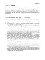
Figure 14.7 illustrates the eight different fragmentations of one m×n multiplica-

tion explored by the algorithm to obtain one k ×p multiplication fragment.
Fig. 14.7 Multiplication fragmentations explored by the algorithm
276 M.C. Molina et al.
14.4.2.4 Transformation of Multiplications into Additions
Due to the given schedule it is not always possible to instance a new multiplier
without exceeding MIWA. Therefore, unallocated multiplications are transformed
into several additions.
14.4.3 Adder Selection and Binding
14.4.3.1 Instantiation and Binding of Adders Without IW
The set of additions considered here may come from the original specification, the
transformation of multiplications (performed in the previous phase), or the transfor-
mation of additions (step 4.3.3). For every different width n of unallocated additions,
the algorithm instances as many adders of that width as the minimum occurrence of
additions of that width per cycle. Next, operations are allocated to them. For every
instanced adder of width n, it calculates the candidates formed by as many additions
of the selected width as the circuit latency, and the IS of every candidate. The algo-
rithm allocates to every adder the operations of the candidate with the highest IS.
The IW of the adders instanced here is zero in all the cycles.
14.4.3.2 Instantiation and Binding of Adders with Some IW
For every different width n of unallocated additions, and from the biggest, the algo-
rithm checks if it is possible to instance one n adder without exceeding MCAAC. It
considers in every cycle the operation (able to be executed over an n adder) that pro-
duces the lowest IW of an n bits adder. After every successful check, the algorithm
instances one adder of the checked width, and allocates operations to it. Now the
candidates are formed by as many operations as the number of cycles where there is
at least one operation that may be executed over one n bits adder. The width of the
candidate operation scheduled in cycle c equals the width of the operation used in
cycle c to perform the check. Once all candidates are calculated, their corresponding
IS are computed, and the additions of the candidate with the highest IS allocated.
Adders instanced in this step may be unused during several cycles, and may also be

used to execute narrower operations (being the IW of these adders in compliance
with MCAAC).
14.4.3.3 Transformation of Additions
This step is only performed when it is not possible to instance a new adder of the
same width as any of the yet unallocated additions without exceeding MCAAC.
Some additions are transformed to obtain one addition fragment of width m from
14 Exploiting Bit-Level Design Techniques in Behavioural Synthesis 277
each of them. These transformations increase the number of m bits additions, which
may result in the final instance of an adder of that width (during previous steps).
First the algorithm selects both the set of the operations to be transformed and the
fragment width, and afterwards it performs the fragmentation of the selected addi-
tions. The fragment size is the minimum width of the widest unallocated operation
scheduled in every cycle. A maximum of one operation per cycle is fragmented each
time, but only in cycles without unallocated operations of the selected width. The
set of fragmented operations is formed by the widest unallocated addition scheduled
in every cycle without operations of the selected width. Every selected addition is
decomposed into two smaller ones, being one of fragments of the desired width.
These fragmentationsproducethe allocation of at least one new adder of the selected
width during the execution of the previous steps, and may also contribute to the
allocation of additional adders.
14.5 Analysis of the Implementations Synthesized Using
the Proposed Techniques
This section presents some of the synthesis results obtained by the algorithms
described previously which include some of the bit level design techniques pro-
posed in this chapter. These results have been compared to those obtained by a HLS
commercial tool, Synopsys Behavioral Compiler (BC) version 2001.08, to evaluate
the quality of the proposed methods and their implementations in HLS algorithms.
The area of the implementations synthesized is measured in number of inverters,
and includes the area of the FUs, storage and routing units, glue logic, and controller.
The clock cycle length is measured in nanoseconds. The RT-level implementations

produced have been translated into VHDL descriptions to be processed by Synopsys
Design Compiler (DC) to obtain the area and time reports. The design library used
in all the experiments is VTVTLIB25 by Virginia Tech. based on 0.25μmTSMC
technology.
14.5.1 Implementation Quality: Influential Factors
The main difference between conventional synthesis algorithms and our approach is
the number of factors that influence the quality of the implementations obtained. The
implementations proposed by conventional algorithms depend on the specification
size, the operation mobility, and the specification heterogeneity, measured as the
number of different triplets (type, data format, width) present in the original specifi-
cation divided by the number of operations. Otherwise, our algorithms minimize the
influence of data dependencies and get implementations totally independent from
the specification heterogeneity, i.e. from the number, type, data format, and width
of the operations used to describe behaviours.
278 M.C. Molina et al.
Just to illustrate these influences we have synthesized different descriptions of the
same behaviour, shown in Table 14.3, first with the proposed algorithms, and after-
wards with BC. These descriptions have been created by progressively transforming
(from circuit A to G) some of the specification operations into several smaller ones,
in order to increase the number of operations of every different type and width, such
that the specification heterogeneities of these descriptions have been progressively
reduced from A to G. Circuit A is the original specification formed by 30 opera-
tions with six different operation types (MAC, multiplication, addition, subtraction,
comparison, and maximum), two different data formats (unsigned and two’s com-
plement), and eight different operation widths (4, 8, 12, 16, 24, 32, 48, and 64 bits).
And circuit G is the specification obtained after the last transformation. It consists
of 86 unsigned multiplications and additions of 26 different widths, thus being the
description with the smallest heterogeneity. Table 14.3 shows the number of opera-
tions (# Operations), the number of different operation types (# Types), the number
of different data formats (# Formats), and the number of different operation widths

(# Widths) present in each synthesized specification. The latency in all cases is equal
to ten cycles. The amount of area saved by the algorithm grows, in general, with the
specification heterogeneity. In the circuits synthesized, the homogeneous distribu-
tion of the computational costs among cycles achieved by our algorithm has also
resulted in substantial clock cycle length reductions. Figure 14.8 shows in this set
of examples the amount of area and clock cycle length saved by our approach in
function of the heterogeneity.
Table 14.3 Features of the synthesized descriptions
Circuit # Operations # Types # Formats # Widths Heterogeneity
A306280.7
B 36 6210 0.55
C 44 5212 0.45
D 52 4115 0.42
E 65 3119 0.35
F 73 3122 0.32
Fig. 14.8 Experimental area and execution time of different descriptions of one specification
14 Exploiting Bit-Level Design Techniques in Behavioural Synthesis 279
Table 14.4 Area results of the synthesis of some modules of the ADPCM decoder algorithm
ADPCM decoder Datapath Commercial tool Fragmentation techniques
module resources (# inverters) (# inverters)
IAQ FUs 388 234
IAQ Controller 60 62
IAQ Multiplexers 158 166
IAQ Registers 189 192
IAQ Total area 798 664 (16.7% saved)
OPFC + SCA FUs 928 478
OPFC + SCA Controller 62 66
OPFC + SCA Multiplexers 418 470
OPFC + SCA Registers 461 475
OPFC + SCA Total area 1,873 1,503 gates (19.7% saved)

TTD FUs 681 285
TTD Controller 60 63
TTD Multiplexers 220 232
TTD Registers 261 273
TTD Total area 1,226 865 (29.4% saved)
Total all modules 3,897 3,032 (22.2% saved)
14.5.2 An Application Example
As an example of a real circuit, we have synthesized the following modules of the
ADPCM decoding algorithm described in the Recommendation G.721 of CCITT:
• Inverse Adaptative Quantizer (IAQ)
• Output PCM Format Conversion (OPFC)
• Synchronous Coding Adjustment (SCA)
• Tone and Transition Detector (TTD)
Table 14.4 compares the area of the modules synthesized by our approach and BC
for a fixed value of the circuit latency. The amount of area saved by our algorithm
averages 22%.
OPFC and SCA modules have been synthesized together,and IAQ and TTD inde-
pendently. Better results could be obtained if all modules were synthesized together,
because it would increase the number of operations that could be executed over the
same FU, and the number of variables that could be stored in the same register.
14.5.3 Synthesis of Non Heterogeneous Specifications
As shown in previous sections, our algorithm substantially reduces the area of cir-
cuits synthesized from heterogeneous specifications, as compared with commercial
tools and previous known approaches. But the application method is not just lim-
ited to heterogeneous specifications. Important area reductions can also be achieved
when specifications formed by operations with the same data formats and widths are