Parallel Programming: for Multicore and Cluster Systems- P6 pdf

40 2 Parallel Computer Architecture
σ : {(x
1
, ,x
d
) | 1 ≤ x
i
≤ n
i
, 1 ≤ i ≤ d}−→{0, 1}
k
with σ ((x
1
, ,x
d
)) = s
1
s
2
s
d
and s
i
= RGC
k
i
(x
i
)
(where s
i

is the x
i
th bit string in the Gray code sequence RGC
k
i
) defines an embed-
ding into the k-dimensional cube. For two mesh nodes (x
1
, ,x
d
) and (y
1
, ,y
d
)
that are connected by an edge in the d-dimensional mesh, there exists exactly one
dimension i ∈{1, ,d} with |x
i
−y
i
|=1 and for all other dimensions j = i,itis
x
j
= y
j
. Thus, for the corresponding hypercube nodes σ ((x
1
, ,x
d
)) = s

1
s
2
s
d
and σ ((y
1
, ,y
d
)) = t
1
t
2
t
d
, all components s
j
= RGC
k
j
(x
j
) = RGC
k
j
(y
j
) =
t
j

for j = i are identical. Moreover, RGC
k
i
(x
i
) and RGC
k
i
(y
i
) differ in exactly one
bit position. Thus, the hypercube nodes s
1
s
2
s
d
and t
1
t
2
t
d
also differ in exactly
one bit position and are therefore connected by an edge in the hypercube network.
2.5.4 Dynamic Interconnection Networks
Dynamic interconnection networks are also called indirect interconnection net-
works. In these networks, nodes or processors are not connected directly with each
other. Instead, switches are used and provide an indirect connection between the
nodes, giving these networks their name. From the processors’ point of view, such a

network forms an interconnection unit into which data can be sent and from which
data can be received. Internally, a dynamic network consists of switches that are
connected by physical links. For a message transmission from one node to another
node, the switches can be configured dynamically such that a connection is estab-
lished.
Dynamic interconnection networks can be characterized according to their topo-
logical structure. Popular forms are bus networks, multistage networks, and crossbar
networks.
2.5.4.1 Bus Networks
A bus essentially consists of a set of wires which can be used to transport data from a
sender to a receiver, see Fig. 2.15 for an illustration. In some cases, several hundreds
12 n
64
m1
I/O
MM
P
C
P
CC
P
12 n
disk
Fig. 2.15 Illustration of a bus network with 64 wires to connect processors P
1
, ,P
n
with caches
C
1

, ,C
n
to memory modules M
1
, ,M
m
2.5 Interconnection Networks 41
of wires are used to ensure a fast transport of large data sets. At each point in time,
only one data transport can be performed via the bus, i.e., the bus must be used in
a time-sharing way. When several processors attempt to use the bus simultaneously,
a bus arbiter is used for the coordination. Because the likelihood for simultaneous
requests of processors increases with the number of processors, bus networks are
typically used for a small number of processors only.
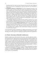
2.5.4.2 Crossbar Networks
An n × m crossbar network has n inputs and m outputs. The actual network con-
sists of n · m switches as illustrated in Fig. 2.16 (left). For a system with a shared
address space, the input nodes may be processors and the outputs may be memory
modules. For a system with a distributed address space, both the input nodes and
the output nodes may be processors. For each request from a specific input to a
specific output, a connection in the switching network is established. Depending
on the specific input and output nodes, the switches on the connection path can
have different states (straight or direction change) as illustrated in Fig. 2.16 (right).
Typically, crossbar networks are used only for a small number of processors because
of the large hardware overhead required.
P
P
MM
P
1
2

n
12
M
m
Fig. 2.16 Illustration of a n ×m crossbar network for n processors and m memory modules (left).
Each network switch can be in one of two states: straight or direction change (right)
2.5.4.3 Multistage Switching Networks
Multistage switching networks consist of several stages of switches with connecting
wires between neighboring stages. The network is used to connect input devices
to output devices. Input devices are typically the processors of a parallel system.
Output devices can be processors (for distributed memory machines) or memory
modules (for shared memory machines). The goal is to obtain a small distance for
arbitrary pairs of input and output devices to ensure fast communication. The inter-
nal connections between the stages can be represented as a graph where switches are
represented by nodes and wires between switches are represented by edges. Input
and output devices can be represented as specialized nodes with edges going into
42 2 Parallel Computer Architecture
the actual switching network graph. The construction of the switching graph and
the degree of the switches used are important characteristics of multistage switching
networks.
Regular multistage interconnection networks are characterized by a regular
construction method using the same degree of incoming and outgoing wires for all
switches. For the switches, a × b crossbars are often used where a is the input
degree and b is the output degree. The switches are arranged in stages such that
neighboring stages are connected by fixed interconnections, see Fig. 2.17 for an
illustration. The input wires of the switches of the first stage are connected with the
input devices. The output wires of the switches of the last stage are connected with
the output devices. Connections from input devices to output devices are performed
by selecting a path from a specific input device to the selected output device and
setting the switches on the path such that the connection is established.

Fig. 2.17 Multistage
interconnection networks
with a × b crossbars as
switches according to [95]
a
b x ab x ab x a
a x b
a x ba x b
a x ba x b
a x b
a
a
a
a
a
a
b
b
b
a
a
processors
fixed interconnections
fixed interconnections
memory modules
The actual graph representing a regular multistage interconnection network
results from gluing neighboring stages of switches together. The connection between
neighboring stages can be described by a directed acyclic graph of depth 1. Using w
nodes for each stage, the degree of each node is g = n/w where n is the number of
edges between neighboring stages. The connection between neighboring stages can

be represented by a permutation π : {1, ,n}→{1, ,n} which specifies which
output link of one stage is connected to which input link of the next stage. This
means that the output links {1, ,n} of one stage are connected to the input links
(π(1), ,π(n)) of the next stage. Partitioning the permutation (π(1), ,π(n))
into w parts results in the ordered set of input links of nodes of the next stage. For
regular multistage interconnection networks, the same permutation is used for all
stages, and the stage number can be used as parameter.
Popular regular multistage networks are the omega network, the baseline net-
work, and the butterfly network. These networks use 2 ×2 crossbar switches which
are arranged in log n stages. Each switch can be in one of four states as illustrated
in Fig. 2.18. In the following, we give a short overview of the omega, baseline,
butterfly, Bene
ˇ
s, and fat tree networks, see [115] for a detailed description.
2.5 Interconnection Networks 43
strai
g
ht crossover upper broadcast lower broadcas
t
Fig. 2.18 Settings for switches in an omega, baseline, or butterfly network
2.5.4.4 Omega Network
An n × n omega network is based on 2 × 2 crossbar switches which are arranged
in log n stages such that each stage contains n/2 switches where each switch has
two input links and two output links. Thus, there are (n/2) ·log n switches in total,
with log n ≡ log
2
n. Each switch can be in one of four states, see Fig. 2.18. In
the omega network, the permutation function describing the connection between
neighboring stages is the same for all stages, independent of the number of the stage.
The switches in the network are represented by pairs (α, i) where α ∈{0, 1}

log n−1
is a bit string of length log n −1 representing the position of a switch within a stage
and i ∈{0, ,log n −1} is the stage number. There is an edge from node (α, i)in
stage i to two nodes (β,i + 1) in stage i + 1 where β is defined as follows:
1. β results from α by a cyclic left shift or
2. β results from α by a cyclic left shift followed by an inversion of the last (right-
most) bit.
An n × n omega network is also called (log n − 1)-dimensional omega network.
Figure 2.19(a) shows a 16×16 (three-dimensional) omega network with four stages
and eight switches per stage.
2.5.4.5 Butterfly Network
Similar to the omega network, a k-dimensional butterfly network connects n = 2
k+1
inputs to n = 2
k+1
outputs using a network of 2 × 2 crossbar switches. Again, the
switches are arranged in k + 1 stages with 2
k
nodes/switches per stage. This results
in a total number (k + 1) · 2
k
of nodes. Again, the nodes are represented by pairs
(α, i) where i for 0 ≤ i ≤ k denotes the stage number and α ∈{0, 1}
k
is the position
of the node in the stage. The connection between neighboring stages i and i +1for
0 ≤ i < k is defined as follows: Two nodes (α, i) and (α

, i + 1) are connected if
and only if

1. α and α

are identical (straight edge) or
2. α and α

differ in precisely the (i + 1)th bit from the left (cross edge).
Figure 2.19(b) shows a 16 ×16 butterfly network with four stages.
2.5.4.6 Baseline Network
The k-dimensional baseline network has the same number of nodes, edges, and
stages as the butterfly network. Neighboring stages are connected as follows: Node
(α, i) is connected to node (α

, i +1) for 0 ≤ i < k if and only if
44 2 Parallel Computer Architecture
a)
01 32
000
011
110
111
001
010
100
101
stage stage stagestage
000
011
110
111
001

010
100
101
b)
2130
stage stage stage stage
000
011
110
111
001
010
100
101
201 3
c)
stage stage stage stage
Fig. 2.19 Examples for dynamic interconnection networks: (a)16×16 omega network, (b)16×16
butterfly network, (c)16×16 baseline network. All networks are three-dimensional
2.5 Interconnection Networks 45
1. α

results from α by a cyclic right shift on the last k −i bits of α or
2. α

results from α by first inverting the last (rightmost) bit of α and then perform-
ing a cyclic right shift on the last k − i bits.
Figure 2.19(c) shows a 16 ×16 baseline network with four stages.
2.5.4.7 Bene
ˇ

s Network
The k-dimensional Bene
ˇ
s network is constructed from two k-dimensional butterfly
networks such that the first k + 1 stages are a butterfly network and the last k + 1
stages are a reverted butterfly network. The last stage (k + 1) of the first butterfly
network and the first stage of the second (reverted) butterfly network are merged. In
total, the k-dimensional Bene
ˇ
s network has 2k + 1 stages with 2
k
switches in each
stage. Figure 2.20(a) shows a three-dimensional Bene
ˇ
s network as an example.
66543210
000
011
110
111
001
010
100
101
(a)
(b)
Fig. 2.20 Examples for dynamic interconnection networks: (a) three-dimensional Bene
ˇ
snetwork
and (b) fat tree network for 16 processors

2.5.4.8 Fat Tree Network
The basic structure of a dynamic tree or fat tree network is a complete binary tree.
The difference from a normal tree is that the number of connections between the
nodes increases toward the root to avoid bottlenecks. Inner tree nodes consist of
switches whose structure depends on their position in the tree structure. The leaf
level is level 0. For n processors, represented by the leaves of the tree, a switch on
46 2 Parallel Computer Architecture
tree level i has 2
i
input links and 2
i
output links for i = 1, ,log n. This can be
realized by assembling the switches on level i internally from 2
i−1
switches with
two input and two output links each. Thus, each level i consists of n/2 switches in
total, grouped in 2
log n−i
nodes. This is shown in Fig. 2.20(b) for a fat tree with four
layers. Only the inner switching nodes are shown, not the leaf nodes representing
the processors.
2.6 Routing and Switching
Direct and indirect interconnection networks provide the physical basis to send
messages between processors. If two processors are not directly connected by a
network link, a path in the network consisting of a sequence of nodes has to be
used for message transmission. In the following, we give a short description of how
to select a suitable path in the network (routing) and how messages are handled at
intermediate nodes on the path (switching).
2.6.1 Routing Algorithms
A routing algorithm determines a path in a given network from a source node A to a

destination node B. The path consists of a sequence of nodes such that neighboring
nodes in the sequence are connected by a physical network link. The path starts
with node A and ends at node B. A large variety of routing algorithms have been
proposed in the literature, and we can only give a short overview in the following.
For a more detailed description and discussion, we refer to [35, 44].
Typically, multiple message transmissions are being executed concurrently accord-
ing to the requirements of one or several parallel programs. A routing algorithm tries
to reach an even load on the physical network links as well as to avoid the occurrence
of deadlocks. A set of messages is in a deadlock situation if each of the messages is
supposed to be transmitted over a link that is currently used by another message of
the set. A routing algorithm tries to select a path in the network connecting nodes A
and B such that minimum costs result, thus leading to a fast message transmission
between A and B. The resulting communication costs depend not only on the length
of the path used, but also on the load of the links on the path. The following issues
are important for the path selection:
• Network topology: The topology of the network determines which paths are
available in the network to establish a connection between nodes A and B.
• Network contention: Contention occurs when two or more messages should be
transmitted at the same time over the same network link, thus leading to a delay
in message transmission.
• Network congestion: Congestion occurs when too many messages are assigned
to a restricted resource (like a network link or buffer) such that arriving messages
2.6 Routing and Switching 47
have to be discarded since they cannot be stored anywhere. Thus, in contrast to
contention, congestion leads to an overflow situation with message loss [139].
A large variety of routing algorithms have been proposed in the literature. Several
classification schemes can be used for a characterization. Using the path length,
minimal and non-minimal routing algorithms can be distinguished. Minimal rout-
ing algorithms always select the shortest message transmission, which means that
when using a link of the path selected, a message always gets closer to the target

node. But this may lead to congestion situations. Non-minimal routing algorithms
do not always use paths with minimum length if this is necessary to avoid congestion
at intermediate nodes.
A further classification can be made by distinguishing deterministic routing
algorithms and adaptive routing algorithms. A routing algorithm is deterministic if
the path selected for message transmission only depends on the source and destina-
tion nodes regardless of other transmissions in the network. Therefore, deterministic
routing can lead to unbalanced network load. Path selection can be done source
oriented at the sending node or distributed during message transmission at inter-
mediate nodes. An example for deterministic routing is dimension-order routing
which can be applied for network topologies that can be partitioned into several
orthogonal dimensions as is the case for meshes, tori, and hypercube topologies.
Using dimension-order routing, the routing path is determined based on the position
of the source node and the target node by considering the dimensions in a fixed
order and traversing a link in the dimension if necessary. This can lead to network
contention because of the deterministic path selection.
Adaptive routing tries to avoid such contentions by dynamically selecting the
routing path based on load information. Between any pair of nodes, multiple paths
are available. The path to be used is dynamically selected such that network traffic
is spread evenly over the available links, thus leading to an improvement of network
utilization. Moreover, fault tolerance is provided, since an alternative path can be
used in case of a link failure. Adaptive routing algorithms can be further catego-
rized into minimal and non-minimal adaptive algorithms as described above. In the
following, we give a short overview of important routing algorithms. For a more
detailed treatment, we refer to [35, 95, 44, 115, 125].
2.6.1.1 Dimension-Order Routing
We give a short description of XY routing for two-dimensional meshes and E-cube
routing for hypercubes as typical examples for dimension-order routing algorithms.
XY Routing for Two-Dimensional Meshes
For a two-dimensional mesh, the position of the nodes can be described by an X-

coordinate and a Y -coordinate where X corresponds to the horizontal and Y cor-
responds to the vertical direction. To send a message from a source node A with
position (X
A
, Y
A
) to target node B with position (X
B
, Y
B
), the message is sent from
48 2 Parallel Computer Architecture
the source node into (positive or negative) X-direction until the X-coordinate X
B
of B is reached. Then, the message is sent into Y -direction until Y
B
is reached. The
length of the resulting path is | X
A
− X
B
|+|Y
A
−Y
B
|. This routing algorithm is
deterministic and minimal.
E-Cube Routing for Hypercubes
In a k-dimensional hypercube, each of the n = 2
k

nodes has a direct interconnection
link to each of its k neighbors. As introduced in Sect. 2.5.2, each of the nodes can
be represented by a bit string of length k such that the bit string of one of the k
neighbors is obtained by inverting one of the bits in the bit string. E-cube uses the
bit representation of a sending node A and a receiving node B to select a routing
path between them. Let α = α
0
α
k−1
be the bit representation of A and β =
β
0
β
k−1
be the bit representation of B. Starting with A, in each step a dimension
is selected which determines the next node on the routing path. Let A
i
with bit
representation γ = γ
0
γ
k−1
be a node on the routing path A = A
0
, A
1
, ,A
l
=
B from which the message should be forwarded in the next step. For the forwarding

from A
i
to A
i+1
, the following two substeps are made:
• The bit string γ ⊕β is computed where ⊕denotes the bitwise exclusive or com-
putation (i.e., 0 ⊕0 = 0, 0 ⊕1 = 1, 1 ⊕0 = 1, 1 ⊕1 = 0).
• The message is forwarded in dimension d where d is the rightmost bit position
of γ ⊕ β with value 1. The next node A
i+1
on the routing path is obtained by
inverting the dth bit in γ , i.e., the bit representation of A
i+1
is δ = δ
0
δ
k−1
with δ
j
= γ
j
for j = d and δ
d
= ¯γ
d
. The target node B is reached when
γ ⊕β = 0.
Example For k = 3, let A with bit representation α = 010 be the source node and
B with bit representation β = 111 be the target node. First, the message is sent from
A into direction d = 2toA

1
with bit representation 011 (since α ⊕β = 101). Then,
the message is sent in dimension d = 0toβ since (011 ⊕111 = 100).
2.6.1.2 Deadlocks and Routing Algorithms
Usually, multiple messages are in transmission concurrently. A deadlock occurs if
the transmission of a subset of the messages is blocked forever. This can happen in
particular if network resources can be used only by one message at a time. If, for
example, the links between two nodes can be used by only one message at a time
and if a link can only be released when the following link on the path is free, then
the mutual request for links can lead to a deadlock. Such deadlock situations can be
avoided by using a suitable routing algorithm. Other deadlock situations that occur
because of limited size of the input or output buffer of the interconnection links or
because of an unsuited order of the send and receive operations are considered in
Sect. 2.6.3 on switching strategies and Chap. 5 on message-passing programming.
To prove the deadlock freedom of routing algorithms, possible dependencies
between interconnection channels are considered. A dependence from an intercon-
2.6 Routing and Switching 49
nection channel l
1
to an interconnection channel l
2
exists, if it is possible that the
routing algorithm selects a path which contains channel l
2
directly after channel
l
1
. These dependencies between interconnection channels can be represented by a
channel dependence graph which contains the interconnection channels as nodes;
each dependence between two channels is represented by an edge. A routing algo-

rithm is deadlock free for a given topology, if the channel dependence graph does not
contain cycles. In this case, no communication pattern can ever lead to a deadlock.
For topologies that do not contain cycles, no channel dependence graph can
contain cycles, and therefore each routing algorithm for such a topology must be
deadlock free. For topologies with cycles, the channel dependence graph must be
analyzed. In the following, we show that XY routing for two-dimensional meshes
with bidirectional links is deadlock free.
Deadlock Freedom of XY Routing
The channel dependence graph for XY routing contains a node for each uni-
directional link of the two-dimensional n
X
× n
Y
mesh, i.e., there are two nodes
for each bidirectional link of the mesh. There is a dependence from link u to link
v,ifv can be directly reached from u in horizontal or vertical direction or by a 90
◦
(deg) turn down or up. To show the deadlock freedom, all unidirectional links of the
mesh are numbered as follows:
• Each horizontal edge from node (i, y) to node (i + 1, y) gets number i + 1for
i = 0, ,n
x
−2 for each valid value of y. The opposite edge from (i +1, y)to
(i, y) gets number n
x
− 1 − (i + 1) = n
x
− i − 2fori = 0, ,n
x
− 2. Thus,

the edges in increasing x-direction are numbered from 1 to n
x
− 1, the edges in
decreasing x-direction are numbered from 0 to n
x
−2.
• Each vertical edge from (x, j)to(x, j+1) gets number j+n
x
for j = 0, ,n
y
−
2. The opposite edge from (x, j + 1) to (x, j) gets number n
x
+n
y
−( j + 1).
Figure 2.21 shows a 3 × 3 mesh and the resulting channel dependence graph for
XY routing. The nodes of the graph are annotated with the numbers assigned to
the corresponding network links. It can be seen that all edges in the channel depen-
dence graph go from a link with a smaller number to a link with a larger number.
Thus, a delay during message transmission along a routing path can occur only if
the message has to wait after the transmission along a link with number i for the
release of a successive link w with number j > i currently used by another mes-
sage transmission (delay condition). A deadlock can only occur if a set of messages
{N
1
, ,N
k
} and network links {n
1

, ,n
k
} exists such that for 1 ≤ i < k each
message N
i
uses a link n
i
for transmission and waits for the release of link n
i+1
which is currently used for the transmission of message N
i+1
. Additionally, N
k
is
currently transmitted using link n
k
and waits for the release of n
1
used by N
1
.Ifn()
denotes the numbering of the network links introduced above, the delay condition
implies that for the deadlock situation just described, it must be
n(n
1
) < n(n
2
) < ···< n(n
k
) < n(n

1
).