Parallel Programming: for Multicore and Cluster Systems- P13 ppt

3.3 Levels of Parallelism 111
When employing the client–server model for the structuring of parallel programs,
multiple client threads are used which generate requests to a server and then perform
some computations on the result, see Fig. 3.5 (right) for an illustration. After having
processed a request of a client, the server delivers the result back to the client.
The client–server model can be applied in many variations: There may be sev-
eral server threads or the threads of a parallel program may play the role of both
clients and servers, generating requests to other threads and processing requests
from other threads. Section 6.1.8 shows an example for a Pthreads program using
the client–server model. The client–server model is important for parallel program-
ming in heterogeneous systems and is also often used in grid computing and cloud
computing.
3.3.6.7 Pipelining
The pipelining model describes a special form of coordination of different threads
in which data elements are forwarded from thread to thread to perform different pro-
cessing steps. The threads are logically arranged in a predefined order, T
1
, ,T
p
,
such that thread T
i
receives the output of thread T
i−1
as input and produces an output
which is submitted to the next thread T
i+1
as input, i = 2, ,p − 1. Thread T
1
receives its input from another program part and thread T
p

provides its output to
another program part. Thus, each of the pipeline threads processes a stream of input
data in sequential order and produces a stream of output data. Despite the dependen-
cies of the processing steps, the pipeline threads can work in parallel by applying
their processing step to different data.
The pipelining model can be considered as a special form of functional decompo-
sition where the pipeline threads process the computations of an application algo-
rithm one after another. A parallel execution is obtained by partitioning the data
into a stream of data elements which flow through the pipeline stages one after
another. At each point in time, different processing steps are applied to different
elements of the data stream. The pipelining model can be applied for both shared
and distributed address spaces. In Sect. 6.1, the pipelining pattern is implemented
as Pthreads program.
3.3.6.8 Task Pools
In general, a task pool is a data structure in which tasks to be performed are stored
and from which they can be retrieved for execution. A task comprises computations
to be executed and a specification of the data to which the computations should be
applied. The computations are often specified as a function call. A fixed number of
threads is used for the processing of the tasks. The threads are created at program
start by the main thread and they are terminated not before all tasks have been pro-
cessed. For the threads, the task pool is a common data structure which they can
access to retrieve tasks for execution, see Fig. 3.6 (left) for an illustration. During
the processing of a task, a thread can generate new tasks and insert them into the
112 3 Parallel Programming Models
Thread 3
Thread 2
pool
Thread 4
Thread 1
store

task
retrieve
task
store
store
retrieve
store
task
task
retrieve
task
retrieve
task
task
task
task
producer 1
producer 2
producer 3
consumer 1
consumer 2
consumer 3
data
buffer
retrieve
retrieve
store
store
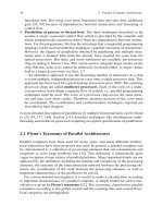
Fig. 3.6 Illustration of a task pool (left) and a producer–consumer model (right)
This

figure
will be
printed
in b/w
task pool. Access to the task pool must be synchronized to avoid race conditions.
Using a task-based execution, the execution of a parallel program is finished, when
the task pool is empty and when each thread has terminated the processing of its
last task. Task pools provide a flexible execution scheme which is especially useful
for adaptive and irregular applications for which the computations to be performed
are not fixed at program start. Since a fixed number of threads is used, the overhead
for thread creation is independent of the problem size and the number of tasks to be
processed.
Flexibility is ensured, since tasks can be generated dynamically at any point dur-
ing program execution. The actual task pool data structure could be provided by
the programming environment used or could be included in the parallel program.
An example for the first case is the Executor interface of Java, see Sect. 6.2 for
more details. A simple task pool implementation based on a shared data structure
is described in Sect. 6.1.6 using Pthreads. For fine-grained tasks, the overhead of
retrieval and insertion of tasks from or into the task pool becomes important, and
sophisticated data structures should be used for the implementation, see [93] for
more details.
3.3.6.9 Producer–Consumer
The producer–consumer model distinguishes between producer threads and con-
sumer threads. Producer threads produce data which are used as input by con-
sumer threads. For the transfer of data from producer threads to consumer threads,
a common data structure is used, which is typically a data buffer of fixed length
and which can be accessed by both types of threads. Producer threads store the
data elements generated into the buffer, consumer threads retrieve data elements
from the buffer for further processing, see Fig. 3.6 (right) for an illustration. A
producer thread can only store data elements into the buffer, if this is not full.

A consumer thread can only retrieve data elements from the buffer, if this is
not empty. Therefore, synchronization has to be used to ensure a correct coor-
dination between producer and consumer threads. The producer–consumer model
is considered in more detail in Sect. 6.1.9 for Pthreads and Sect. 6.2.3 for Java
threads.
3.4 Data Distributions for Arrays 113
3.4 Data Distributions for Arrays
Many algorithms, especially from numerical analysis and scientific computing, are
based on vectors and matrices. The corresponding programs use one-, two-, or
higher dimensional arrays as basic data structures. For those programs, a straight-
forward parallelization strategy decomposes the array-based data into subarrays and
assigns the subarrays to different processors. The decomposition of data and the
mapping to different processors is called data distribution, data decomposition,
or data partitioning. In a parallel program, the processors perform computations
only on their part of the data.
Data distributions can be used for parallel programs for distributed as well as for
shared memory machines. For distributed memory machines, the data assigned to
a processor reside in its local memory and can only be accessed by this processor.
Communication has to be used to provide data to other processors. For shared mem-
ory machines, all data reside in the same shared memory. Still a data decomposition
is useful for designing a parallel program since processors access different parts
of the data and conflicts such as race conditions or critical regions are avoided.
This simplifies the parallel programming and supports a good performance. In this
section, we present regular data distributions for arrays, which can be described by a
mapping from array indices to processor numbers. The set of processors is denoted
as P ={P
1
, ,P
p
}.

3.4.1 Data Distribution for One-Dimensional Arrays
For one-dimensional arrays the blockwise and the cyclic distribution of array ele-
ments are typical data distributions. For the formulation of the mapping, we assume
that the enumeration of array elements starts with 1; for an enumeration starting
with 0 the mappings have to be modified correspondingly.
The blockwise data distribution of an array v = (v
1
, ,v
n
) of length n cuts
the array into p blocks with n/pconsecutive elements each. Block j,1≤ j ≤ p,
contains the consecutive elements with indices ( j − 1) ·n/p+1, , j ·n/p
and is assigned to processor P
j
. When n is not a multiple of p, the last block con-
tains less than n/ p elements. For n = 14 and p = 4 the following blockwise
distribution results:
P
1
:ownsv
1
, v
2
, v
3
, v
4
,
P
2

:ownsv
5
, v
6
, v
7
, v
8
,
P
3
:ownsv
9
, v
10
, v
11
, v
12
,
P
4
:ownsv
13
, v
14
.
Alternatively, the first n mod p processors get n/pelements and all other proces-
sors get n/pelements.
The cyclic data distribution of a one-dimensional array assigns the array ele-

ments in a round robin way to the processors so that array element v
i
is assigned to
processor P
(i−1) mod p +1
, i = 1, ,n. Thus, processor P
j
owns the array elements
114 3 Parallel Programming Models
j, j + p, , j + p ·
(
n/p−1
)
for j ≤ n mod p and j, j + p, , j + p ·
(
n/p−2
)
for n mod p < j ≤ p. For the example n = 14 and p = 4 the cyclic
data distribution
P
1
:ownsv
1
, v
5
, v
9
, v
13
,

P
2
:ownsv
2
, v
6
, v
10
, v
14
,
P
3
:ownsv
3
, v
7
, v
11
,
P
4
:ownsv
4
, v
8
, v
12
results, where P
j

for 1 ≤ j ≤ 2 = 14 mod 4 owns the elements j, j + 4, j +4 ∗
2, j +4 ∗(4 −1) and P
j
for 2 < j ≤ 4 owns the elements j, j +4, j +4 ∗(4 −2).
The block–cyclic data distribution is a combination of the blockwise and cyclic
distributions. Consecutive array elements are structured into blocks of size b, where
b  n/p in most cases. When n is not a multiple of b, the last block contains
less than b elements. The blocks of array elements are assigned to processors in a
round robin way. Figure 3.7a shows an illustration of the array decompositions for
one-dimensional arrays.
3.4.2 Data Distribution for Two-Dimensional Arrays
For two-dimensional arrays, combinations of blockwise and cyclic distributions in
only one or both dimensions are used.
For the distribution in one dimension, columns or rows are distributed in a block-
wise, cyclic, or block–cyclic way. The blockwise columnwise (or rowwise) distribu-
tion builds p blocks of contiguous columns (or rows) of equal size and assigns block
i to processor P
i
, i = 1, ,p. When n is not a multiple of p, the same adjustment
as for one-dimensional arrays is used. The cyclic columnwise (or rowwise) distri-
bution assigns columns (or rows) in a round robin way to processors and uses the
adjustments of the last blocks as described for the one-dimensional case, when n is
not a multiple of p. The block–cyclic columnwise (or rowwise) distribution forms
blocks of contiguous columns (or rows) of size b and assigns these blocks in a round
robin way to processors. Figure 3.7b illustrates the distribution in one dimension for
two-dimensional arrays.
A distribution of array elements of a two-dimensional array of size n
1
×n
2

in both
dimensions uses checkerboard distributions which distinguish between blockwise
cyclic and block–cyclic checkerboard patterns. The processors are arranged in a
virtual mesh of size p
1
· p
2
= p where p
1
is the number of rows and p
2
is the
number of columns in the mesh. Array elements (k, l) are mapped to processors
P
i,j
, i = 1, , p
1
, j = 1, , p
2
.
In the blockwise checkerboard distribution, the array is decomposed into
p
1
· p
2
blocks of elements where the row dimension (first index) is divided into
p
1
blocks and the column dimension (second index) is divided into p
2

blocks.
Block (i, j), 1 ≤ i ≤ p
1
,1 ≤ j ≤ p
2
, is assigned to the processor with
position (i, j) in the processor mesh. The block sizes depend on the number of
rows and columns of the array. Block (i, j) contains the array elements (k, l) with
k = (i−1)·n
1
/p
1
+1, ,i·n
1
/p
1
and l = ( j−1)·n
2
/p
2
+1, , j ·n
2
/p
2
.
Figure 3.7c shows an example for n
1
= 4, n
2
= 8, and p

1
· p
2
= 2 ·2 = 4.
3.4 Data Distributions for Arrays 115
887654321 1234567
8101191234567 12
887654321 1234567
3
1
2
4
3
1
2
4
8101191234567 12
3
1
2
4
887654321 1234567
3
1
2
4
3
1
2
4

8101191234567 12
3
1
2
4
P
PP
P
12
34
P
PP
P
12
34
P
PP
P
12
34
P
PP
P
12
34
P
PP
P
12
34

P
PP
P
12
34
P
PP
P
12
34
P
PP
P
12
34
a)
c)
b)
PP
PP
PPPP
PPPPPP
PPPPPPPP
131234
123412
PPPPPP P PPPPP
PPPPPP
1234 131234
123412
1

4
1234 4
2
2
4
PP
PP
12
4
PP
PP
12
4
PP
PP
12
4
3
33
2
3
cilcyc esiwkcolb
block−cyclic
cilcyc esiwkcolb
block−cyclic
cilcyc esiwkcolb
block−cyclic
Fig. 3.7 Illustration of the data distributions for arrays: (a) for one-dimensional arrays, (b)for
two-dimensional arrays within one of the dimensions, and (c) for two-dimensional arrays with
checkerboard distribution

The cyclic checkerboard distribution assigns the array elements in a round
robin way in both dimensions to the processors in the processor mesh so that a
cyclic assignment of row indices k = 1, ,n
1
to mesh rows i = 1, , p
1
and a
cyclic assignment of column indices l = 1, ,n
2
to mesh columns j = 1, , p
2
result. Array element (k, l) is thus assigned to the processor with mesh position
116 3 Parallel Programming Models
((k − 1) mod p
1
+1, (l −1) mod p
2
+1). When n
1
and n
2
are multiples of p
1
and
p
2
, respectively, the processor at position (i, j) owns all array elements (k,l) with
k = i +s·p
1
and l = j +t ·p

2
for 0 ≤ s < n
1
/p
1
and 0 ≤ t < n
2
/p
2
. An alternative
way to describe the cyclic checkerboard distribution is to build blocks of size p
1
×p
2
and to map element (i, j) of each block to the processor at position (i, j)inthemesh.
Figure 3.7c shows a cyclic checkerboard distribution with n
1
= 4, n
2
= 8, p
1
= 2,
and p
2
= 2. When n
1
or n
2
is not a multiple of p
1

or p
2
, respectively, the cyclic
distribution is handled as in the one-dimensional case.
The block–cyclic checkerboard distribution assigns blocks of size b
1
× b
2
cyclically in both dimensions to the processors in the following way: Array element
(m, n) belongs to the block (k, l), with k =m/b
1
 and l =n/b
2
. Block (k, l)is
assigned to the processor at mesh position ((k −1) mod p
1
+1, (l −1) mod p
2
+1).
The cyclic checkerboard distribution can be considered as a special case of the
block–cyclic distribution with b
1
= b
2
= 1, and the blockwise checkerboard dis-
tribution can be considered as a special case with b
1
= n
1
/p

1
and b
2
= n
2
/p
2
.
Figure 3.7c illustrates the block–cyclic distribution for n
1
= 4, n
2
= 12, p
1
= 2,
and p
2
= 2.
3.4.3 Parameterized Data Distribution
A data distribution is defined for a d-dimensional array A with index set I
A
⊂
N
d
. The size of the array is n
1
×···×n
d
and the array elements are denoted as
A[i

1
, ,i
d
] with an index i = (i
1
, ,i
d
) ∈ I
A
. Array elements are assigned to
p processors which are arranged in a d-dimensional mesh of size p
1
×···× p
d
with p =

d
i=1
p
i
. The data distribution of A is given by a distribution function
γ
A
: I
A
⊂ N
d
→ 2
P
, where 2

P
denotes the power set of the set of processors P.
The meaning of γ
A
is that the array element A[i
1
, ,i
d
] with i = (i
1
, ,i
d
)is
assigned to all processors in γ
A
(i) ⊆ P, i.e., array element A[i] can be assigned
to more than one processor. A data distribution is called replicated,ifγ
A
(i) = P
for all i ∈ I
A
. When each array element is uniquely assigned to a processor, then
|γ
A
(i)|=1 for all i ∈ I
A
; examples are the block–cyclic data distribution described
above. The function L(γ
A
):P → 2

I
A
delivers all elements assigned to a specific
processor, i.e.,
i ∈ L(γ
A
)(q) if and only if q ∈ γ
A
(i).
Generalizations of the block–cyclic distributions in the one- or two-dimensional
case can be described by a distribution vector in the following way. The array
elements are structured into blocks of size b
1
, ,b
d
where b
i
is the block size
in dimension i, i = 1, ,d. The array element A[i
1
, ,i
d
] is contained in
block (k
1
, ,k
d
) with k
j
=i

j
/b
j
 for 1 ≤ j ≤ d. The block (k
1
, ,k
d
)is
then assigned to the processor at mesh position ((k
1
− 1) mod p
1
+ 1, ,(k
d
−
1) mod p
d
+ 1). This block–cyclic distribution is called parameterized data dis-
tribution with distribution vector
3.5 Information Exchange 117
(
(p
1
, b
1
), ,(p
d
, b
d
)

)
. (3.1)
This vector uniquely determines a block–cyclic data distribution for a d-dimensional
array of arbitrary size. The blockwise and the cyclic distributions of a d-dimensional
array are special cases of this distribution. Parameterized data distributions are used
in the applications of later sections, e.g., the Gaussian elimination in Sect. 7.1.
3.5 Information Exchange
To control the coordination of the different parts of a parallel program, informa-
tion must be exchanged between the executing processors. The implementation of
such an information exchange strongly depends on the memory organization of the
parallel platform used. In the following, we give a first overview on techniques for
information exchange for shared address space in Sect. 3.5.1 and for distributed
address space in Sect. 3.5.2. More details will be discussed in the following chapters.
As example, parallel matrix–vector multiplication is considered for both memory
organizations in Sect. 3.6.
3.5.1 Shared Variables
Programming models with a shared address space are based on the existence of a
global memory which can be accessed by all processors. Depending on the model,
the executing control flows may be referred to as processes or threads, see Sect. 3.7
for more details. In the following, we will use the notation threads, since this is more
common for shared address space models. Each thread will be executed by one pro-
cessor or by one core for multicore processors. Each thread can access shared data
in the global memory. Such shared data can be stored in shared variables which
can be accessed as normal variables. A thread may also have private data stored in
private variables, which cannot be accessed by other threads. There are different
ways how parallel program environments define shared or private variables. The
distinction between shared and private variables can be made by using annotations
like shared or private when declaring the variables. Depending on the pro-
gramming model, there can also be declaration rules which can, for example, define
that global variables are always shared and local variables of functions are always

private. To allow a coordinated access to a shared variable by multiple threads,
synchronization operations are provided to ensure that concurrent accesses to the
same variable are synchronized. Usually, a sequentialization is performed such
that concurrent accesses are done one after another. Chapter 6 considers program-
ming models and techniques for shared address spaces in more detail and describes
different systems, like Pthreads, Java threads, and OpenMP. In the current section, a
few basic concepts are given for a first overview.
118 3 Parallel Programming Models
A central concept for information exchange in shared address space is the use
of shared variables. When a thread T
1
wants to transfer data to another thread T
2
,
it stores the data in a shared variable such that T
2
obtains the data by reading this
shared variable. To ensure that T
2
reads the variable not before T
1
has written the
appropriate data, a synchronization operation is used. T
1
stores the data into the
shared variable before the corresponding synchronization point and T
2
reads the
data after the synchronization point.
When using shared variables, multiple threads accessing the same shared variable

by a read or write at the same time must be avoided, since this may lead to race
conditions. The term race condition describes the effect that the result of a parallel
execution of a program part by multiple execution units depends on the order in
which the statements of the program part are executed by the different units. In the
presence of a race condition it may happen that the computation of a program part
leads to different results, depending on whether thread T
1
executes the program part
before T
2
or vice versa. Usually, race conditions are undesirable, since the relative
execution speed of the threads may depend on many factors (like execution speed
of the executing cores or processors, the occurrence of interrupts, or specific values
of the input data) which cannot be influenced by the programmer. This may lead
to non-deterministic behavior, since, depending on the execution order, different
results are possible, and the exact outcome cannot be predicted.
Program parts in which concurrent accesses to shared variables by multiple
threads may occur, thus holding the danger of the occurrence of inconsistent values,
are called critical sections. An error-free execution can be ensured by letting only
one thread at a time execute a critical section. This is called mutual exclusion.Pro-
gramming models for shared address space provide mechanisms to ensure mutual
exclusion. The techniques used have originally been developed for multi-tasking
operating systems and have later been adapted to the needs of parallel programming
environments. For a concurrent access of shared variables, race conditions can be
avoided by a lock mechanism, which will be discussed in more detail in Sect. 3.7.3.
3.5.2 Communication Operations
In programming models with a distributed address space, exchange of data and
information between the processors is performed by communication operations
which are explicitly called by the participating processors. The execution of such
a communication operation causes one processor to receive data that is stored in

the local memory of another processor. The actual data exchange is realized by
the transfer of messages between the participating processors. The corresponding
programming models are therefore called message-passing programming models.
To send a message from one processor to another, one send and one receive
operations have to be used as a pair. A send operation sends a data block from the
local address space of the executing processor to another processor as specified by
the operation. A receive operation receives a data block from another processor and
3.5 Information Exchange 119
stores it in the local address space of the executing processor. This kind of data
exchange is also called point-to-point communication, since there is exactly one
send point and one receive point. Additionally, global communication operations
are often provided in which a larger set of processors is involved. These global
communication operations typically capture a set of regular communication patterns
often used in parallel programs [19, 100].
3.5.2.1 A Set of Communication Operations
In the following, we consider a typical set of global communication operations
which will be used in the following chapters to describe parallel implementations for
platforms with a distributed address space [19]. We consider p identical processors
P
1
, ,P
p
and use the index i, i ∈{1, , p}, as processor rank to identify the
processor P
i
.
• Single transfer: For a single transfer operation, a processor P
i
(sender) sends
a message to processor P

j
(receiver) with j = i. Only these two processors
participate in this operation. To perform a single transfer operation, P
i
executes
a send operation specifying a send buffer in which the message is provided as
well as the processor rank of the receiving processor. The receiving processor
P
j
executes a corresponding receive operation which specifies a receive buffer to
store the received message as well as the processor rank of the processor from
which the message should be received. For each send operation, there must be
a corresponding receive operation, and vice versa. Otherwise, deadlocks may
occur, see Sects. 3.7.4.2 and 5.1.1 for more details. Single transfer operations are
the basis of each communication library. In principle, any communication pattern
can be assembled with single transfer operations. For regular communication pat-
terns, it is often beneficial to use global communication operations, since they are
typically easier to use and more efficient.
• Single-broadcast: For a single-broadcast operation, a specific processor P
i
sends
the same data block to all other processors. P
i
is also called root in this context.
The effect of a single-broadcast operation with processor P
1
as root and message
x can be illustrated as follows:
P
1

: x P
1
: x
P
2
: - P
2
: x
.
.
.
broadcast
=⇒
.
.
.
P
p
: - P
p
: x
Before the execution of the broadcast, the message x is only stored in the local
address space of P
1
. After the execution of the operation, x is also stored in
the local address space of all other processors. To perform the operation, each
processor explicitly calls a broadcast operation which specifies the root processor
of the broadcast. Additionally, the root processor specifies a send buffer in which
120 3 Parallel Programming Models
the broadcast message is provided. All other processors specify a receive buffer

in which the message should be stored upon receipt.
• Single-accumulation: For a single-accumulation operation, each processor pro-
vides a block of data with the same type and size. By performing the operation,
a given reduction operation is applied element by element to the data blocks
provided by the processors, and the resulting accumulated data block of the
same length is collected at a specific root processor P
i
. The reduction oper-
ation is a binary operation which is associative and commutative. The effect
of a single-accumulation operation with root processor P
1
to which each pro-
cessor P
i
provides a data block x
i
for i = 1, ,p can be illustrated as
follows:
P
1
: x
1
P
1
: x
1
+ x
2
+···+x
p

P
2
: x
2
P
2
: x
2
.
.
.
accumulation
=⇒
.
.
.
P
p
: x
p
P
p
: x
p
The addition is used as reduction operation. To perform a single-accumulation,
each processor explicitly calls the operation and specifies the rank of the root pro-
cessor, the reduction operation to be applied, and the local data block provided.
The root processor additionally specifies the buffer in which the accumulated
result should be stored.
• Gather: For a gather operation, each processor provides a data block, and the data

blocks of all processors are collected at a specific root processor P
i
. No reduction
operation is applied, i.e., processor P
i
gets p messages. For root processor P
1
,
the effect of the operation can be illustrated as follows:
P
1
: x
1
P
1
: x
1
 x
2
···x
p
P
2
: x
2
P
2
: x
2
.

.
.
gather
=⇒
.
.
.
P
p
: x
p
P
p
: x
p
Here, the symbol || denotes the concatenation of the received data blocks. To
perform the gather, each processor explicitly calls a gather operation and speci-
fies the local data block provided as well as the rank of the root processor. The
root processor additionally specifies a receive buffer in which all data blocks are
collected. This buffer must be large enough to store all blocks. After the operation
is completed, the receive buffer of the root processor contains the data blocks of
all processors in rank order.
• Scatter: For a scatter operation, a specific root processor P
i
provides a sepa-
rate data block for every other processor. For root processor P
1
, the effect of the
operation can be illustrated as follows: