Parallel Programming: for Multicore and Cluster Systems- P14 ppt

3.5 Information Exchange 121
P
1
: x
1
 x
2
···x
p
P
1
: x
1
P
2
: - P
2
: x
2
.
.
.
scatter
=⇒
.
.
.
P
p
: - P
p

: x
p
To perform the scatter, each processor explicitly calls a scatter operation and
specifies the root processor as well as a receive buffer. The root processor addi-
tionally specifies a send buffer in which the data blocks to be sent are provided
in rank order of the rank i = 1, ,p.
• Multi-broadcast: The effect of a multi-broadcast operation is the same as the
execution of several single-broadcast operations, one for each processor, i.e., each
processor sends the same data block to every other processor. From the receiver’s
point of view, each processor receives a data block from every other processor.
Different receivers get the same data block from the same sender. The operation
can be illustrated as follows:
P
1
: x
1
P
1
: x
1
 x
2
···x
p
P
2
: x
2
P
2

: x
1
 x
2
···x
p
.
.
.
multi-broadcast
=⇒
.
.
.
P
p
: x
p
P
p
: x
1
 x
2
···x
p
In contrast to the global operations considered so far, there is no root processor.
To perform the multi-broadcast, each processor explicitly calls a multi-broadcast
operation and specifies a send buffer which contains the data block as well as
a receive buffer. After the completion of the operation, the receive buffer of

every processor contains the data blocks provided by all processors in rank order,
including its own data block. Multi-broadcast operations are useful to collect
blocks of an array that have been computed in a distributed way and to make the
entire array available to all processors.
• Multi-accumulation: The effect of a multi-accumulation operation is that each
processor executes a single-accumulation operation, i.e., each processor provides
for every other processor a potentially different data block. The data blocks for
the same receiver are combined with a given reduction operation such that one
(reduced) data block arrives at the receiver. There is no root processor, since each
processor acts as a receiver for one accumulation operation. The effect of the
operation with addition as reduction operation can be illustrated as follows:
P
1
: x
11
 x
12
···x
1p
P
1
: x
11
+ x
21
+···+x
p1
P
2
: x

21
 x
22
···x
2p
P
2
: x
12
+ x
22
+···+x
p2
.
.
.
multi-accumulation
=⇒
.
.
.
P
p
: x
p1
 x
p2
···x
pp
P

p
: x
1p
+ x
2p
+···+x
pp
122 3 Parallel Programming Models
The data block provided by processor P
i
for processor P
j
is denoted as x
ij
, i, j =
1, ,p. To perform the multi-accumulation, each processor explicitly calls a
multi-accumulation operation and specifies a send buffer, a receive buffer, and a
reduction operation. In the send buffer, each processor provides a separate data
block for each other processor, stored in rank order. After the completion of the
operation, the receive buffer of each processor contains the accumulated result
for this processor.
• Total exchange: For a total exchange operation, each processor provides for each
other processor a potentially different data block. These data blocks are sent to
their intended receivers, i.e., each processor executes a scatter operation. From
a receiver’s point of view, each processor receives a data block from each other
processor. In contrast to a multi-broadcast, different receivers get different data
blocks from the same sender. There is no root processor. The effect of the opera-
tion can be illustrated as follows:
P
1

: x
11
 x
12
···x
1p
P
1
: x
11
 x
21
···x
p1
P
2
: x
21
 x
22
···x
2p
P
2
: x
12
 x
22
···x
p2

.
.
.
total exchange
=⇒
.
.
.
P
p
: x
p1
 x
p2
···x
pp
P
p
: x
1p
 x
2p
···x
pp
To perform the total exchange, each processor specifies a send buffer and a
receive buffer. The send buffer contains the data blocks provided for the other
processors in rank order. After the completion of the operation, the receive buffer
of each processor contains the data blocks gathered from the other processors in
rank order.
Section 4.3.1 considers the implementation of these global communication oper-

ations for different networks and derives running times. Chapter 5 describes how
these communication operations are provided by the MPI library.
3.5.2.2 Duality of Communication Operations
A single-broadcast operation can be implemented by using a spanning tree with the
sending processor as root. Edges in the tree correspond to physical connections in
the underlying interconnection network. Using a graph representation G = (V, E)
of the network, see Sect. 2.5.2, a spanning tree can be defined as a subgraph G

=
(V, E

) which contains all nodes of V and a subset E

⊆ E of the edges such that
E

represents a tree. The construction of a spanning tree for different networks is
considered in Sect. 4.3.1.
Given a spanning tree, a single-broadcast operation can be performed by a top-
down traversal of the tree such that starting from the root each node forwards the
message to be sent to its children as soon as the message arrives. The message can
be forwarded over different links at the same time. For the forwarding, the tree edges
can be partitioned into stages such that the message can be forwarded concurrently
3.5 Information Exchange 123
PP
PPP
PP
P
P
0

0
1
1
22
1
1
26
4
357
98
1
P
234
P
PP
8
89
67
45
98
PP
P
P
9
3
5
7
P
aa
a

a
6
745
2
3
i
a
Σ
i=1
a
9
a +a +a +a
a +a +a
a +a +a +a
89
1
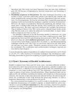
Fig. 3.8 Implementation of a single-broadcast operation using a spanning tree (left). The edges
of the tree are annotated with the stage number.Theright tree illustrates the implementation of a
single-accumulation with the same spanning tree. Processor P
i
provides a value a
i
for i = 1, ,9.
The result is accumulated at the root processor P
1
[19]
over all edges of a stage. Figure 3.8 (left) shows a spanning tree with root P
1
and
three stages 0, 1, 2.

Similar to a single-broadcast, a single-accumulation operation can also be imple-
mented by using a spanning tree with the accumulating processor as root. The reduc-
tion is performed at the inner nodes according to the given reduction operation. The
accumulation results from a bottom-up traversal of the tree, see Fig. 3.8 (right). Each
node of the spanning tree receives a data block from each of its children (if present),
combines these blocks according to the given reduction operation, including its own
data block, and forwards the results to its parent node. Thus, one data block is sent
over each edge of the spanning tree, but in the opposite direction as has been done
for a single-broadcast. Since the same spanning trees can be used, single-broadcast
and single-accumulation are dual operations.
A duality relation also exists between a gather and a scatter operation as well as
between a multi-broadcast and a multi-accumulation operation.
A scatter operation can be implemented by a top-down traversal of a spanning
tree where each node (except the root) receives a set of data blocks from its parent
node and forwards those data blocks that are meant for a node in a subtree to its
corresponding child node being the root of that subtree. Thus, the number of data
blocks forwarded over the tree edges decreases on the way from the root to the
leaves. Similarly, a gather operation can be implemented by a bottom-up traversal
of the spanning tree where each node receives a set of data blocks from each of its
child nodes (if present) and forwards all data blocks received, including its own
data block, to its parent node. Thus, the number of data blocks forwarded over
the tree edges increases on the way from the leaves to the root. On each path to
the root, over each tree edge the same number of data blocks are sent as for a
scatter operation, but in opposite direction. Therefore, gather and scatter are dual
operations. A multi-broadcast operation can be implemented by using p spanning
trees where each spanning tree has a different root processor. Depending on the
124 3 Parallel Programming Models
underlying network, there may or may not be physical network links that are used
multiple times in different spanning trees. If no links are shared, a transfer can be
performed concurrently over all spanning trees without waiting, see Sect. 4.3.1 for

the construction of such sets of spanning trees for different networks. Similarly, a
multi-accumulation can also be performed by using p spanning trees, but compared
to a multi-broadcast, the transfer direction is reversed. Thus, multi-broadcast and
multi-accumulation are also dual operations.
3.5.2.3 Hierarchy of Communication Operations
The communication operations described form a hierarchy in the following way:
Starting from the most general communication operation (total exchange), the other
communication operations result by a stepwise specialization. A total exchange is
the most general communication operation, since each processor sends a potentially
different message to each other processor. A multi-broadcast is a special case of
a total exchange in which each processor sends the same message to each other,
i.e., instead of p different messages, each processor provides only one message. A
multi-accumulation is also a special case of a total exchange for which the messages
arriving at an intermediate node are combined according to the given reduction
operation before they are forwarded. A gather operation with root P
i
is a special
case of a multi-broadcast which results from considering only one of the receiving
processors, P
i
, which receives a message from every other processor. A scatter
operation with root P
i
is a special case of multi-accumulation which results by
using a special reduction operation which forwards the messages of P
i
and ignores
all other messages. A single-broadcast is a special case of a scatter operation in
total exchange
duality

duality
duality
single transfer
multi-broadcast operation
scatter operation
single-broadcast operation
multi-accumulation operation
gather operation
single-accumulation operation
Fig. 3.9 Hierarchy of global communication operations. The horizontal arrows denote duality
relations. The dashed arrows show specialization relations [19]
3.6 Parallel Matrix–Vector Product 125
which the root processor sends the same message to every other processor, i.e.,
instead of p different messages the root processor provides only one message. A
single-accumulation is a special case of a gather operation in which a reduction is
performed at intermediate nodes of the spanning tree such that only one (combined)
message results at the root processor. A single transfer between processors P
i
and
P
j
is a special case of a single-broadcast with root P
i
for which only the path from
P
i
to P
j
is relevant. A single transfer is also a special case of a single-accumulation
with root P

j
using a special reduction operation which forwards only the message
from P
i
. In summary, the hierarchy in Fig. 3.9 results.
3.6 Parallel Matrix–Vector Product
The matrix–vector multiplication is a frequently used component in scientific com-
puting. It computes the product Ab = c, where A ∈ R
n×m
is an n × m matrix
and b ∈ R
m
is a vector of size m. (In this section, we use bold-faced type for the
notation of matrices or vectors and normal type for scalar values.) The sequential
computation of the matrix–vector product
c
i
=
m

j=1
a
ij
b
j
, i = 1, , n,
with c = (c
1
, ,c
n

) ∈ R
n
, A = (a
ij
)
i=1, ,n, j=1, ,m
, and b = (b
1
, ,b
m
), can be
implemented in two ways, differing in the loop order of the loops over i and j. First,
the matrix–vector product is considered as the computation of n scalar products
between rows a
1
, ,a
n
of A and vector b, i.e.,
A · b =
⎛
⎜
⎝
(a
1
, b)
.
.
.
(a
n

, b)
⎞
⎟
⎠
,
where (x, y) =

m
j=1
x
j
y
j
for x, y ∈ R
m
with x = (x
1
, ,x
m
) and y =
(y
1
, ,y
m
) denotes the scalar product (or inner product) of two vectors. The cor-
responding algorithm (in C notation) is
for (i=0; i<n; i++) c[i] = 0;
for (i=0; i<n; i++)
for (j=0; j<m; j++)
c[i] = c[i] + A[i][j]

*
b[j];
The matrix A ∈ R
n×m
is implemented as a two-dimensional array A and the vectors
b ∈ R
m
and c ∈ R
n
are implemented as one-dimensional arrays b and c.(The
indices start with 0 as usual in C.) For each i = 0, ,n-1, the inner loop
body consists of a loop over j computing one of the scalar products. Second, the
126 3 Parallel Programming Models
matrix–vector product can be written as a linear combination of columns
˜
a
1
, ,
˜
a
m
of A with coefficients b
1
, ,b
m
, i.e.,
A · b =
m

j=1

b
j
˜
a
j
.
The corresponding algorithm (in C notation) is:
for (i=0; i<n; i++) c[i] = 0;
for (j=0; j<m; j++)
for (i=0; i<n; i++)
c[i] = c[i] + A[i][j]
*
b[j] ;
For each j = 0, ,m-1, a column
˜
a
j
is added to the linear combination.
Both sequential programs are equivalent since there are no dependencies and the
loops over i and j can be exchanged. For a parallel implementation, the row- and
column-oriented representations of matrix A give rise to different parallel imple-
mentation strategies.
(a) The row-oriented representation of matrix A in the computation of n scalar
products (a
i
, b), i = 1, ,n,ofrowsofA with vector b leads to a parallel
implementation in which each processor of a set of p processors computes
approximately n/p scalar products.
(b) The column-oriented representation of matrix A in the computation of the
linear combination


m
j=1
b
j
˜
a
j
of columns of A leads to a parallel implemen-
tation in which each processor computes a part of this linear combination with
approximately m/ p column vectors.
In the following, we consider these parallel implementation strategies for the case
of n and m being multiples of the number of processors p.
3.6.1 Parallel Computation of Scalar Products
For a parallel implementation of a matrix–vector product on a distributed memory
machine, the data distribution of A and b is chosen such that the processor comput-
ing the scalar product (a
i
, b), i ∈{1, ,n}, accesses only data elements stored in
its private memory, i.e., row a
i
of A and vector b are stored in the private memory
of the processor computing the corresponding scalar product. Since vector b ∈ R
m
is needed for all scalar products, b is stored in a replicated way. For matrix A,a
row-oriented data distribution is chosen such that a processor computes the scalar
product for which the matrix row can be accessed locally. Row-oriented blockwise
as well as cyclic or block–cyclic data distributions can be used.
For the row-oriented blockwise data distribution of matrix A, processor P
k

, k =
1, ,p, stores the rows a
i
, i = n/p · (k − 1) + 1, ,n/p · k, in its private
memory and computes the scalar products (a
i
, b). The computation of (a
i
, b) needs
3.6 Parallel Matrix–Vector Product 127
no data from other processors and, thus, no communication is required. According
to the row-oriented blockwise computation the result vector c = (c
1
, ,c
n
) has a
blockwise distribution.
When the matrix–vector product is used within a larger algorithm like iteration
methods, there are usually certain requirements for the distribution of c. In iteration
methods, there is often the requirement that the result vector c has the same data
distribution as the vector b. To achieve a replicated distribution for c, each proces-
sor P
k
, k = 1, , p, sends its block (c
n/p·(k−1)+1
, ,c
n/p·k
) to all other proces-
sors. This can be done by a multi-broadcast operation. A parallel implementation
of the matrix–vector product including this communication is given in Fig. 3.10.

The program is executed by all processors P
k
, k = 1, , p, in the SPMD style.
The communication operation includes an implicit barrier synchronization. Each
processor P
k
stores a different part of the n ×m array A in its local array local A
of dimension local
n × m. The block of rows stored by P
k
in local A contains
the global elements
local
A[i][j]=A[i+(k-1)
*
n/p][j]
with i = 0, ,n/p − 1, j = 0, ,m − 1, and k = 1, ,p. Each processor
computes a local matrix–vector product of array local
A with array b and stores
the result in array local
c of size local n. The communication operation
multi
broadcast(local c,local n,c)
performs a multi-broadcast operation with the local arrays local
c of all proces-
sors as input. After this communication operation, the global array c contains the
values
c[i+(k-1)
*
n/p]=local

c[i]
for i = 0, ,n/ p − 1 and k = 1, , p, i.e., the array c contains the values of
the local vectors in the order of the processors and has a replicated data distribution.
Fig. 3.10 Program fragment in C notation for a parallel program of the matrix–vector product with
row-oriented blockwise distribution of the matrix A and a final redistribution of the result vector c
128 3 Parallel Programming Models
See Fig. 3.13(1) for an illustration of the data distribution of A, b, and c for the
program given in Fig. 3.10.
For a row-oriented cyclic distribution, each processor P
k
, k = 1, , p,stores
the rows a
i
of matrix A with i = k + p ·(l − 1) for l = 1, ,n/ p and computes
the corresponding scalar products. The rows in the private memory of processor P
k
are stored within one local array local A of dimension local n ×m.Afterthe
parallel computation of the result array local
c, the entries have to be reordered
correspondingly to get the global result vector in the original order.
For the implementation of the matrix–vector product on a shared memory
machine, the row-oriented distribution of the matrix A and the corresponding dis-
tribution of the computation can be used. Each processor of the shared memory
machine computes a set of scalar products as described above. A processor P
k
com-
putes n/p elements of the result vector c and uses n/p corresponding rows of matrix
A in a blockwise or cyclic way, k = 1, , p. The difference to the implementation
on a distributed memory machine is that an explicit distribution of the data is not
necessary since the entire matrix A and vector b reside in the common memory

accessible by all processors.
The distribution of the computation to processors according to a row-oriented
distribution, however, causes the processors to access different elements of A and
compute different elements of c. Thus, the write accesses to c cause no conflict.
Since the accesses to matrix A and vector b are read accesses, they also cause
no conflict. Synchronization and locking are not required for this shared memory
implementation. Figure 3.11 shows an SPMD program for a parallel matrix–vector
multiplication accessing the global arrays A, b, and c. The variable k denotes the
processor id of the processor P
k
, k = 1, ,p. Because of this processor number
k, each processor P
k
computes different elements of the result array c. The pro-
gram fragment ends with a barrier synchronization synch() to guarantee that all
processors reach this program point and the entire array c is computed before any
processor executes subsequent program parts. (The same program can be used for a
distributed memory machine when the entire arrays A, b, and c are allocated in
each private memory; this approach needs much more memory since the arrays are
allocated p times.)
Fig. 3.11 Program fragment in C notation for a parallel program of the matrix–vector prod-
uct with row-oriented blockwise distribution of the computation. In contrast to the pro-
gram in Fig. 3.10, the program uses the global arrays A, b, and c for a shared memory
system
3.6 Parallel Matrix–Vector Product 129
3.6.2 Parallel Computation of the Linear Combinations
For a distributed memory machine, the parallel implementation of the matrix–vector
product in the form of the linear combination uses a column-oriented distribution of
the matrix A. Each processor computes the part of the linear combination for which
it owns the corresponding columns

˜
a
i
, i ∈{1, ,m}. For a blockwise distribution
of the columns of A, processor P
k
owns the columns
˜
a
i
, i = m/p · (k − 1) +
1, ,m/ p · k, and computes the n-dimensional vector
d
k
=
m/p·k

j=m/p·(k−1)+1
b
j
˜
a
j
,
which is a partial linear combination and a part of the total result, k = 1, ,p.For
this computation only a block of elements of vector b is accessed and only this block
needs to be stored in the private memory. After the parallel computation of the vec-
tors d
k
, k = 1, ,p, these vectors are added to give the final result c =


p
k=1
d
k
.
Since the vectors d
k
are stored in different local memories, this addition requires
communication, which can be performed by an accumulation operation with the
addition as reduction operation. Each of the processors P
k
provides its vector d
k
for
the accumulation operation. The result of the accumulation is available on one of
the processors. When the vector is needed in a replicated distribution, a broadcast
operation is performed. The data distribution before and after the communication
is illustrated in Fig. 3.13(2a). A parallel program in the SPMD style is given in
Fig. 3.12. The local arrays local
b and local A store blocks of b and blocks of
columns of A so that each processor P
k
owns the elements
local
A[i][j]=A[i][j+(k-1)
*
m/p]
and
local

b[j]=b[j+(k-1)
*
m/p],
Fig. 3.12 Program fragment in C notation for a parallel program of the matrix–vector product
with column-oriented blockwise distribution of the matrix A and reduction operation to compute
the result vector c. The program uses local array d for the parallel computation of partial linear
combinations
130 3 Parallel Programming Models
where j=0, ,m/p-1, i=0, ,n-1, and k=1, ,p. The array d is a
private vector allocated by each of the processors in its private memory containing
different data after the computation. The operation
single
accumulation(d,local m,c,ADD,1)
denotes an accumulation operation, for which each processor provides its array d of
size n, and ADD denotes the reduction operation. The last parameter is 1 and means
that processor P
1
is the root processor of the operation, which stores the result of the
addition into the array c of length n. The final single
broadcast(c,1) sends
the array c from processor P
1
to all other processors and a replicated distribution of
c results.
Alternatively to this final communication, multi-accumulation operation can be
applied which leads to a blockwise distribution of array c. This program version
may be advantageous if c is required to have the same distribution as array b. Each
processor accumulates the n/p elements of the local arrays d, i.e., each processor
computes a block of the result vector c and stores it in its local memory. This com-
munication is illustrated in Fig. 3.13(2b).

For shared memory machines, the parallel computation of the linear combina-
tions can also be used but special care is needed to avoid access conflicts for the
write accesses when computing the partial linear combinations. To avoid write con-
flicts, a separate array d
k of length n should be allocated for each of the processors
P
k
to compute the partial result in parallel without conflicts. The final accumulation
needs no communication, since the data d
k are in the common memory, and can
be performed in a blocked way.
The computation and communication time for the matrix–vector product is ana-
lyzed in Sect. 4.4.2.
3.7 Processes and Threads
Parallel programming models are often based on processors or threads. Both are
abstractions for a flow of control, but there are some differences which we will
consider in this section in more detail. As described in Sect. 3.2, the principal idea
is to decompose the computation of an application into tasks and to employ multi-
ple control flows running on different processors or cores for their execution, thus
obtaining a smaller overall execution time by parallel processing.
3.7.1 Processes
In general, a process is defined as a program in execution. The process comprises the
executable program along with all information that is necessary for the execution
of the program. This includes the program data on the runtime stack or the heap,