Parallel Programming: for Multicore and Cluster Systems- P44 pdf

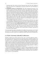
7.4 Conjugate Gradient Method 423
processor performs the arithmetic operations locally and the vector x
k+1
results
in a blockwise distribution.
(4) The axpy-operation g
k+1
= g
k
+α
k
w
k
is computed analogously to computation
step (3) and the result vector g
k+1
is distributed in a blockwise way.
(5) The scalar product γ
k+1
= g
T
k+1
g
k+1
is computed analogously to computation
step (2). The resulting scalar value β
k
is computed by the root processor of a
single-accumulation operation and then broadcasted to all other processors.
(6) The axpy-operation d
k+1

=−g
k+1
+β
k
d
k
is computed analogously to compu-
tation step (3). The result vector d
k+1
has a blockwise distribution.
7.4.2.3 Parallel Execution Time
The parallel execution time of one iteration step of the CG method is the sum of
the parallel execution times of the basic operations involved. We derive the paral-
lel execution time for p processors; n is the system size. It is assumed that n is a
multiple of p. The parallel execution time of one axpy-operation is given by
T
axpy
= 2 ·
n
p
·t
op
,
since each processor computes n/p components and the computation of each com-
ponent needs one multiplication and one addition. As in earlier sections, the time for
one arithmetic operation is denoted by t
op
. The parallel execution time of a scalar
product is
T

scal prod
= 2 ·

n
p
−1

·t
op
+ T
acc
(+)(p, 1) + T
sb
(p, 1) ,
where T
acc
(op)(p, m) denotes the communication time of a single-accumulation
operation with reduction operation op on p processors and message size m.The
computation of the local scalar products with n/ p components requires n/ p multi-
plications and n/p −1 additions. The distribution of the result of the parallel scalar
product, which is a scalar value, i.e., has size 1, needs the time of a single-broadcast
operation T
sb
(p, 1). The matrix–vector multiplication needs time
T
math vec mult
= 2 ·
n
2
p

·t
op
,
since each processor computes n/p scalar products. The total computation time of
the CG method is
T
CG
= T
mb

p,
n
p

+ T
math vec mult
+2 · T
scal prod
+3 · T
axpy
,
424 7 Algorithms for Systems of Linear Equations
where T
mb
(p, m) is the time of a multi-broadcast operation with p processors and
message size m. This operation is needed for the re-distribution of the direction
vector d
k
from iteration step k .
7.5 Cholesky Factorization for Sparse Matrices

Linear equation systems arising in practice are often large but have sparse coef-
ficient matrices, i.e., they have many zero entries. For sparse matrices with regu-
lar structure, like banded matrices, only the diagonals with non-zero elements are
stored and the solution methods introduced in the previous sections can be used. For
an unstructured pattern of non-zero elements in sparse matrices, however, a more
general storage scheme is needed and other parallel solution methods are applied.
In this section, we consider the Cholesky factorization as an example of such a
solution method. The general sequential factorization algorithm and its variants for
sparse matrices are introduced in Sect. 7.5.1. A specific storage scheme for sparse
unstructured matrices is given in Sect. 7.5.2. In Sect. 7.5.3, we discuss parallel
implementations of sparse Cholesky factorization for shared memory machines.
7.5.1 Sequential Algorithm
The Cholesky factorization is a direct solution method for a linear equation system
Ax = b. The method can be used if the coefficient matrix A = (a
ij
) ∈ R
n×n
is
symmetric and positive definite, i.e., if a
ij
= a
ji
and x
T
Ax > 0 for all x ∈ R
n
with
x = 0. For a symmetric and positive definite n × n matrix A ∈ R
n×n
there exists a

unique triangular factorization
A = LL
T
, (7.59)
where L = (l
ij
)
i, j=1, ,n
is a lower triangular matrix, i.e., l
ij
= 0fori < j and
i, j ∈{1, ,n}, with positive diagonal elements, i.e., l
ii
> 0fori = 1, ,n;
L
T
denotes the transposed matrix of L, i.e., L
T
= (l
T
ij
)
i, j=1, ,n
with l
T
ij
= l
ji
[166].
Using the factorization in Eq. (7.59), the solution x of a system of equations Ax = b

with b ∈ R
n
is determined in two steps by solving the triangular systems Ly = b
and L
T
x = y one after another. Because of Ly = LL
T
x = Ax = b, the vector
x ∈ R
n
is the solution of the given linear equation system.
The implementation of the Cholesky factorization can be derived from a column-
wise formulation of A = LL
T
. Comparing the elements of A and LL
T
, we obtain
a
ij
=
n

k=1
l
ik
l
T
kj
=
n


k=1
l
ik
l
jk
=
j

k=1
l
ik
l
jk
=
j

k=1
l
jk
l
ik
7.5 Cholesky Factorization for Sparse Matrices 425
since l
jk
= 0fork > j and by exchanging elements in the last summation. Denoting
the columns of A as
˜
a
1

, ,
˜
a
n
and the columns of L as
˜
l
1
, ,
˜
l
n
results in an
equality for column
˜
a
j
= (a
1 j
, ,a
nj
) and columns
˜
l
k
= (l
1k
, ,l
nk
)fork ≤ j:

˜
a
j
=
j

k=1
l
jk
˜
l
k
leading to
l
jj
˜
l
j
=
˜
a
j
−
j−1

k=1
l
jk
˜
l

k
(7.60)
for j = 1, ,n. If the columns
˜
l
k
, k = 1, , j −1, are already known, the right-
hand side of Formula (7.60) is computable and the column
˜
l
j
can also be computed.
Thus, the columns of L are computed one after another. The computation of column
˜
l
j
has two cases:
For the diagonal element the computation is
l
jj
l
jj
= a
jj
−
j−1

k=1
l
jk

l
jk
or l
jj
=




a
jj
−
j−1

k=1
l
2
jk
.
For the elements l
ij
, i > j, the computation is
l
ij
=
1
l
jj

a

ij
−
j−1

k=1
l
jk
l
ik

;
The elements in the upper triangular of matrix L are l
ij
= 0fori < j.
The Cholesky factorization yields the factorization A = LL
T
for a given matrix
A [65] by computing L = (l
ij
)
i=0, ,n−1, j=0, ,i
from A = (a
ij
)
i, j=0, ,n−1
column
by column from left to right according to the following algorithm, in which the
numbering starts with 0:
(I)
for (j=0; j<n; j++) {

l
jj
=

a
jj
−
j−1

k=0
l
2
jk
;
for (i=j+1; i<n; i++)
l
ij
=
1
l
jj

a
ij
−
j−1

k=0
l
jk

l
ik

;
}
426 7 Algorithms for Systems of Linear Equations
*
*
*
j
*
*
*
*
*
*
j
j
*
*
*
j
*
*
*
*
*
*
j
data items used for the computation

Computation structure
for computing l
ij
Computation structure
for left-looking strategy
Computation structure
for right-looking strategy
*
*
*
j
i
*
*
*
*
*
*
data items updated in the computation
Fig. 7.22 Computational structures and data dependences for the computation of L according
to the basic algorithm (left), the left-looking algorithm (middle), and the right-looking algorithm
(right)
For each column j, first the new diagonal element l
jj
is computed using the elements
in row j; then, the new elements of column j are computed using row j of A and
all columns i of L with i < j, see Fig. 7.22 (left).
For dense matrices A, the Cholesky factorization requires O(n
2
) storage space

and O(n
3
/6) arithmetic operations [166]. For sparse matrices, drastic reductions in
storage and execution time can be achieved by exploiting the sparsity of A, i.e., by
storing and computing only the non-zero entries of A.
The Cholesky factorization usually causes fill-ins for sparse matrices A which
means that the matrix L has non-zeros in positions which are zero in A. The number
of fill-in elements can be reduced by reordering the rows and columns of A result-
inginamatrixPAP
T
with a corresponding permutation matrix P. For Cholesky
factorization, P can be chosen without regard to numerical stability, because no
pivoting is required [65]. Since PAP
T
is also symmetric and positive definite for
any permutation matrix P, the factorization of A can be done with the following
steps:
1. Reordering: Find a permutation matrix P ∈ R
n×n
that minimizes the storage
requirement and computing time by reducing fill-ins. The reordered linear equa-
tion system is (PAP
T
)(Px) = Pb.
2. Storage allocation: Determine the structure of the matrix L and set up the sparse
storage scheme. This is done before the actual computation of L and is called
(symbolic factorization), see [65].
3. Numerical factorization: Perform the factorization PAP
T
= LL

T
.
4. Triangular solution: Solve Ly = Pb and L
T
z = y. Then, the solution of the
original system is x = P
T
z.
The problem of finding an ordering that minimizes the amount of fill-in is
NP-complete [177]. But there exist suitable heuristics for reordering. The most
7.5 Cholesky Factorization for Sparse Matrices 427
popular sequential fill-in reduction heuristic is the minimum degree algorithm [65].
Symbolic factorization by a graph-theoretic approach is described in detail in [65].
In the following, we concentrate on the numerical factorization, which is considered
to require by far the most computation time, and assume that the coefficient matrix
is already in reordered form.
7.5.1.1 Left-Looking Algorithms
According to [124], we denote the sparsity structure of column j and row i of L
(excluding diagonal entries) by
Struct(L
∗j
) ={k > j|l
kj
= 0}
Struct(L
i∗
) ={k < i|l
ik
= 0}
Struct(L

∗j
) contains the row indices of all non-zeros of column j and Struct(L
i∗
)
contains the column indices of all non-zeros of row i. Using these sparsity structures
a slight modification of computation scheme (I) results. The modification uses the
following procedures for manipulating columns [124, 152]:
(II)
cmod(j,k) =
for each i ∈ Struct(L
∗k
) with i ≥ j :
a
ij
= a
ij
−l
jk
l
ik
;
cdiv(j) =
l
jj
=
√
a
jj
;
for each i ∈ Struct(L

∗j
) :
l
ij
= a
ij
/l
jj
;
Procedure cmod( j, k) modifies column j by subtracting a multiple with factor l
jk
of column k from column j for columns k already computed. Only the non-zero
elements of column k are considered in the computation. The entries a
ij
of the
original matrix a are now used to store the intermediate results of the computa-
tion of L. Procedure cdiv ( j) computes the square root of the diagonal element and
divides all entries of column j by this square root of its diagonal entry l
jj
.Using
these two procedures, column j can be computed by applying cmod( j, k) for each
k ∈ Struct(L
j∗
) and then completing the entries by applying cdiv( j). Applying
cmod(j, k) to columns k ∈ Struct(L
j∗
) has no effect because l
jk
= 0. The columns
of L are computed from left to right and the computation of a column

˜
l
j
needs
all columns
˜
l
k
to the left of column
˜
l
j
. This results in the following left-looking
algorithm:
428 7 Algorithms for Systems of Linear Equations
(III)
left cholesky =
for j = 0, , n − 1 {
for each k ∈ Struct(L
j∗
):
cmod( j, k);
cdiv( j);
}
The code in scheme (III) computes the columns one after another from left to
right. The entries of column j are modified after all columns to the left of j have
completely been computed, i.e., the same target column j is used for a number of
consecutive cmod(j, k) operations; this is illustrated in Fig. 7.22 (middle).
7.5.1.2 Right-Looking Algorithm
An alternative way is to use the entries of column j after the complete computation

of column j to modify all columns k to the right of j that depend on column j, i.e.,
to modify all columns k ∈ Struct(L
∗j
) by subtracting l
kj
times the column j from
column k. Because l
kj
= 0fork /∈ Struct(L
∗j
), only the columns k ∈ Struct(L
∗j
)
are manipulated by column j. Still the columns are computed from left to right. The
difference to the left-looking algorithm is that the calls to cmod() for a column j
are done earlier. The final computation of a column j then consists only of a call
to cdiv( j) after all columns to the left are computed. This results in the following
right-looking algorithm:
(IV)
right cholesky =
for j = 0, , n − 1 {
cdiv( j);
for each k ∈ Struct(L
∗j
):
cmod(k, j);
}
The code fragment shows that in the right-looking algorithm, successive cmod()
operations manipulate different target columns with the same column j. An illus-
tration is given in Fig. 7.22 (right).

In both the left-looking and right-looking algorithms, each non-zero l
ij
leads to
an execution of a cmod() operation. In the left-looking algorithm, the cmod(j, k)
operation is used to compute column j. In the right-looking algorithm, the
cmod(k, j) operation is used to manipulate column k ∈ Struct(L
∗j
) after the com-
putation of column j. Thus, left-looking and right-looking algorithms use the same
number of cmod() operations. They also use the same number of cdiv() operations,
since there is exactly one cdiv() operation for each column.
7.5 Cholesky Factorization for Sparse Matrices 429
7.5.1.3 Supernodes
The supernodal algorithm is a computation scheme for sparse Cholesky factoriza-
tion that exploits similar patterns of non-zero elements in adjacent columns, see
[124, 152]. A supernode is a set
I(p) ={p, p +1, , p +q −1}
of contiguous columns in L for which for all i with p ≤ i ≤ p +q −1
Struct(L
∗i
) = Struct(L
∗(p+q−1)
) ∪{i + 1, , p + q − 1} .
Thus, a supernode has a dense triangular block above (and including) row p +q −1,
i.e., all entries are non-zero elements, and an identical sparsity structure for each
column below row p+q−1, i.e., each column has its non-zero elements in the same
rows as the other columns in the supernode. Figure 7.23 shows an example. Because
of this identical sparsity structure of the columns, a supernode has the property that
each member column modifies the same set of target columns outside its supernode
[152]. Thus, the factorization can be expressed in terms of supernodes modifying

columns, rather than columns modifying columns.
0123456789
0
1
2
3
4
5
6
7
8
9
∗
∗∗
∗
∗∗
∗∗∗
∗
∗∗∗ ∗
∗∗∗∗ ∗∗
∗∗
∗∗∗∗ ∗∗∗∗
9
8
5
7
61
04
3
2

Fig. 7.23 Matrix L with supernodes I (0) ={0}, I(1) ={1}, I(2) ={2, 3, 4}, I(5) ={5}, I(6) =
{6, 7}, I(8) ={8, 9}. The elimination tree is shown at the right
Using the definitions first(J) = p and last(J) = p + q − 1 for a supernode
J = I (p) ={p, p +1, ,p +q −1}, the following additional procedure smod()
is defined:
(V)
smod( j, J) =
r = min{j − 1, last(J)};
for k = first(J), ,r
cmod( j, k);
430 7 Algorithms for Systems of Linear Equations
which modifies column j with all columns from supernode J . There are two cases
for modifying a column with a supernode: When column j belongs to supernode J,
then column j is modified only by those columns of J that are to the left in node J.
When column j does not belong to supernode J, then column j is modified by all
columns of J. Using the procedure smod(), the Cholesky factorization can be per-
formed by the following computation scheme, also called right-looking supernodal
algorithm:
(VI)
supernode cholesky =
for each supernode J do from left to right {
cdiv( first(J ));
for j = first(J) +1, ,last(J) {
smod( j, J);
cdiv( j);
}
for k ∈ Struct(L
∗(last(J))
)
smod(k, J);

}
This computation scheme still computes the columns of L from left to right. The
difference to the algorithms presented before is that the computations associated
with a supernode are combined. On the supernode level, a right-looking scheme is
used: For the computation of the first column of a supernode J only one cdiv()
operation is necessary when the modification with all columns to the left is already
done. The columns of J are computed in a left-looking way: After the computa-
tion of all supernodes to the left of supernode J and because the columns of J are
already modified with these supernodes due the supernodal right-looking scheme,
column j is computed by first modifying it with all columns of J to the left of j
and then performing a cdiv() operation. After the computation of all columns of
J, all columns k to the right of J that depend on columns of J are modified with
each column in J , i.e., by the procedure smod(k, J).
An alternative way would be a right-looking computation of the columns of J.
An advantage of the supernodal algorithm lies in an increased locality of memory
accesses because each column of a supernode J is used for the modification of
several columns to the right of J and because all columns of J areusedforthe
modification of the same columns to the right of J .
7.5.2 Storage Schemefor Sparse Matrices
Since most entries in a sparse matrix are zero, specific storage schemes are used
to avoid the storage of zero elements. These compressed storage schemes store the
non-zero entries and additional information about the row and column indices to
7.5 Cholesky Factorization for Sparse Matrices 431
identify its original position in the full matrix. Thus, a compressed storage scheme
for sparse matrices needs the space for the non-zero elements as well as space for
additional information.
A sparse lower triangular matrix L is stored in a compressed storage scheme of
size O(n+nz) where n is the number of rows (or columns) in L and nz is the number
of non-zeros. We present the storage scheme of the SPLASH implementation which,
according to [116], stores a sparse matrix in a compressed manner similar to [64].

This storage scheme exploits the sparsity structure as well as the supernode structure
to store the data. We first describe a simpler version using only the sparsity structure
without supernodes. Exploiting the supernode structure is then based on this storage
scheme.
The storage scheme uses two arrays Nonzero and Row of length nz and
three arrays StartColumn, StartRow, and Supernode of length n. The array
Nonzero contains the values of all non-zeros of a triangular matrix L = (l
kj
)
k≥j
in column-major order, i.e., the non-zeros are ordered columnwise from left to
right in a linear array. Information about the corresponding column indices of non-
zero elements is implicitly contained in array StartColumn: Position j of array
StartColumn stores the index of array Nonzero in which the first non-zero
element of column j is stored, i.e., Nonzero[StartColumn[ j]] contains l
jj
.
Because the non-zero elements are stored columnwise, StartColumn[ j +1] −1
contains the last non-zero element of column j. Thus, the non-zeros of the jth
column of L are assigned to the contiguous part of array Nonzero with indices
from StartColumn[ j]toStartColumn[ j +1] −1. The size of the contiguous
part of non-zeros of column j in array Nonzero is N
j
:= StartColumn[ j +
1]−StartColumn[ j]. The array Row contains the row indices of the correspond-
ing elements in Nonzero. In the simpler version without supernodes, Row[r] con-
tains the row index of the non-zero stored in Nonzero[r], r = 0, ,nz − 1.
Corresponding to the blockwise storage scheme in Nonzero, the indices of the
non-zeros of one column are stored in a contiguous block in Row.
When the similar sparsity structure of rows in the same supernode is addi-

tionally exploited, row indices of non-zeros are stored in a combination of the
arrays Row and StartRow in the following way: StartRow[ j] stores the index
of Row in which the row index of the first non-zero of column j is stored, i.e.,
Row[StartRow[ j]] = j because l
jj
is the first non-zero. For each column the row
indices are still stored in a contiguous block of Row. In contrast to the simpler
scheme the blocks for different rows in the same supernode are not disjoint but
overlap according to the similar sparsity structure of those columns.
The additional array StartRow can be used for a more compact storage scheme
for the supernodal algorithm. When j is the first column of a supernode I( j) =
{j, j + 1, , j + k − 1}, then column j + l for 1 ≤ l < k has the same non-zero
pattern as row j for rows greater than or equal to j +l, i.e., Row[StartRow[ j]+l]
contains the row index of the first element of column j +l. Since this is the diagonal
element, Row[StartRow[ j] + l] = j + l holds. The next entries are the row
indices of the other non-zero elements of column j + l. Thus, the row indices of
column j + l are stored in Row[StartRow[ j] + l], ,Row[StartRow[ j] +
432 7 Algorithms for Systems of Linear Equations
r
j
+N
j
−1
r
j
+N
j
−1
N
j

=c
j+1
c−
j
0
column j
0
1
2
StartColumn Nonzero
Row StartRow
l
l
l
l
00
11
j j
j+1,j+1
nz−1,nz−1
l
c
c
c
c
c
0
1
j
j+1

n−1
k
k
k
0
k
r
1
r
j
r
n−1r
n−1
r
j
r
r
r
r
r
0
1
j
j+1
n−1
0
1
j
j+1
n−1

r
j+1
j+1
r
c
c
c
c
j+1
nz−1
0
1
j
j
+1
n−1
j
1
Struct(L
*j
)
k
non−zeros of
= number of non−zeros in column j
Fig. 7.24 Compressed storage scheme for a sparse lower triangular matrix L.ThearrayNonzero
contains the non-zero elements of matrix L and the array StartColumn contains the positions
of the first elements of columns in Nonzero. The array Row contains the row indices of elements
in Nonzero; the first element of a row is given in StartRow. For a supernodal algorithm, Row
can additionally use an overlapping storage (not shown here)
StartColumn[ j+1]−StartColumn[ j−1]]. This leads to StartRow[ j+l] =

StartRow[ j] +l and thus only the row indices of the first column of a supernode
have to be stored to get the full information. A fast access to the sets Struct(L
∗j
)is
given by
Struct(L
∗j
) =

Row[StartRow[ j] +i]|0≤i≤StartColumn[j +1]
− StartColumn[ j − 1]

.
The storage scheme is illustrated in Fig. 7.24. The array Supernode is used for
the management of supernodes: If a column j is the first column of a supernode J,
then the number of columns of J is stored in Supernode[j].
7.5.3 Implementation for Shared Variables
For a parallel implementation of sparse Cholesky factorization, we consider a shared
memory machine. There are several sources of parallelism for sparse Cholesky fac-
torization, including fine-grained parallelism within the single operations cmod( j, k)
or cdiv(j) as well as column-oriented parallelism in the left-looking, right-looking,
and supernodal algorithms.
The sparsity structure of L may lead to an additional source of parallelism which
is not available for dense factorization. Data dependences may be avoided when
different columns (and the columns having effect on them) have a disjoint spar-
sity structure. This kind of parallelism can be described by elimination trees that