cơ khí liên tục và dẻo
Bạn đang xem bản rút gọn của tài liệu. Xem và tải ngay bản đầy đủ của tài liệu tại đây (7.08 MB, 685 trang )
Continuum
Mechanics
and Plasticity
© 2005 by Chapman & Hall/CRC Press
© 2005 by Chapman & Hall/CRC Press
CRC SERIES: MODERN MECHANICS AND MATHEMATICS
PUBLISHED TITLES
BEYOND PERTURBATION: INTRODUCTION TO THE HOMOTOPY ANALYSIS METHOD
by Shijun Liao
MECHANICS OF ELASTIC COMPOSITES
by Nicolaie Dan Cristescu, Eduard-Marius Craciun, and Eugen Soós
CONTINUUM MECHANICS AND PLASTICITY
by Han-Chin Wu
FORTHCOMING TITLES
HYBRID INCOMPATIBLE FINITE ELEMENT METHODS
by Theodore H.H. Pian, Chang-Chun Wu
MICROSTRUCTURAL RANDOMNESS IN MECHANICS OF MATERIALS
by Martin Ostroja Starzewski
Series Editors: David Gao and Ray W. Ogden
CHAPMAN & HALL/CRC
A CRC Press Company
Boca Raton London New York Washington, D.C.
Han-Chin Wu
Continuum
Mechanics
and Plasticity
© 2005 by Chapman & Hall/CRC Press
This book contains information obtained from authentic and highly regarded sources. Reprinted material
is quoted with permission, and sources are indicated. A wide variety of references are listed. Reasonable
efforts have been made to publish reliable data and information, but the author and the publisher cannot
assume responsibility for the validity of all materials or for the consequences of their use.
Neither this book nor any part may be reproduced or transmitted in any form or by any means, electronic
or mechanical, including photocopying, microfilming, and recording, or by any information storage or
retrieval system, without prior permission in writing from the publisher.
The consent of CRC Press does not extend to copying for general distribution, for promotion, for creating
new works, or for resale. Specific permission must be obtained in writing from CRC Press for such
copying.
Direct all inquiries to CRC Press, 2000 N.W. Corporate Blvd., Boca Raton, Florida 33431.
Trademark Notice: Product or corporate names may be trademarks or registered trademarks, and are
used only for identification and explanation, without intent to infringe.
© 2005 by Chapman & Hall/CRC Press
No claim to original U.S. Government works
International Standard Book Number 1-58488-363-4
Library of Congress Card Number 2004055118
Printed in the United States of America 1 2 3 4 5 6 7 8 9 0
Printed on acid-free paper
Library of Congress Cataloging-in-Publication Data
Wu, Han-Chin.
Continuum mechanics and plasticity / Han-Chin Wu.
p. cm. — (Modern mechanics and mathematics series ; no. 3)
Includes index.
ISBN 1-58488-363-4 (alk. paper)
1. Continuum mechanics. 2. Plasticity. I. Title. II. CRC series—modern mechanics and
mathematics ; 3.
QA808.2.W8 2004
531—dc22 2004055118
© 2005 by Chapman & Hall/CRC Press
Visit the CRC Press Web site at www.crcpress.com
Contents
Preface xiii
Author xvii
Part I Fundamentals of Continuum Mechanics
1 Cartesian Tensors 3
1.1 Introduction 3
1.1.1 Notations 3
1.1.2 Cartesian Coordinate System 4
1.1.3 Special Tensors 4
1.2 Vectors 5
1.2.1 Base Vectors and Components 5
1.2.2 Vector Addition and Multiplication 5
1.2.3 The e–δ Identity 6
1.3 The Transformation of Axes 8
1.4 The Dyadic Product (The Tensor Product) 12
1.5 Cartesian Tensors 13
1.5.1 General Properties 13
1.5.2 Multiplication of Tensors 16
1.5.3 The Component Form and Matrices 18
1.5.4 Quotient Law 19
1.6 Rotation of a Tensor 20
1.6.1 Orthogonal Tensor 20
1.6.2 Component Form of Rotation of a Tensor 22
1.6.3 Some Remarks 23
1.7 The Isotropic Tensors 28
1.8 Vector and Tensor Calculus 34
1.8.1 Tensor Field 34
1.8.2 Gradient, Divergence, Curl 34
1.8.3 The Theorem of Gauss 37
References 40
Problems 41
2 Stress 45
2.1 Introduction 45
2.2 Forces 45
v
© 2005 by Chapman & Hall/CRC Press
vi Contents
2.3 Stress Vector 46
2.4 The Stress Tensor 47
2.5 Equations of Equilibrium 50
2.6 Symmetry of the Stress Tensor 52
2.7 Principal Stresses 53
2.8 Properties of Eigenvalues and Eigenvectors 55
2.9 Normal and Shear Components 59
2.9.1 Directions Along which Normal Components of
σ
ij
Are Maximized or Minimized 60
2.9.2 The Maximum Shear Stress 60
2.10 Mean and Deviatoric Stresses 64
2.11 Octahedral Shearing Stress 65
2.12 The Stress Invariants 66
2.13 Spectral Decomposition of a Symmetric Tensor of Rank Two 69
2.14 Powers of a Tensor 71
2.15 Cayley–Hamilton Theorem 72
References 73
Problems 74
3 Motion and Deformation 79
3.1 Introduction 79
3.2 Material and Spatial Descriptions 80
3.2.1 Material Description 80
3.2.2 Spatial Description 81
3.3 Description of Deformation 83
3.4 Deformation of a Neighborhood 83
3.4.1 Homogeneous Deformations 85
3.4.2 Nonhomogeneous Deformations 86
3.5 The Deformation Gradient 88
3.5.1 The Polar Decomposition Theorem 88
3.5.2 Polar Decompositions of the Deformation Gradient 90
3.6 The Right Cauchy–Green Deformation Tensor 98
3.6.1 The Physical Meaning 98
3.6.2 Transformation Properties of C
RS
101
3.6.3 Eigenvalues and Eigenvectors of C
RS
103
3.6.4 Principal Invariants of C
RS
104
3.7 Deformation of Volume and Area of a Material Element 105
3.8 The Left Cauchy–Green Deformation Tensor 108
3.9 The Lagrangian and Eulerian Strain Tensors 108
3.9.1 Definitions 108
3.9.2 Geometric Interpretation of the Strain Components 112
3.9.3 The Volumetric Strain 115
3.10 Other Strain Measures 118
3.11 Material Rate of Change 119
3.11.1 Material Description of the Material Derivative 119
3.11.2 Spatial Description of the Material Derivative 120
© 2005 by Chapman & Hall/CRC Press
Contents vii
3.12 Dual Vectors and Dual Tensors 122
3.13 Velocity of a Particle Relative to a Neighboring Particle 124
3.14 Physical Significance of the Rate of Deformation Tensor 125
3.15 Physical Significance of the Spin Tensor 128
3.16 Expressions for D and W in Terms of F 129
3.17 Material Derivative of Strain Measures 131
3.18 Material Derivative of Area and Volume Elements 132
References 133
Problems 134
4 Conservation Laws and Constitutive Equation 141
4.1 Introduction 141
4.2 Bulk Material Rate of Change 142
4.3 Conservation Laws 145
4.3.1 The Conservation of Mass 145
4.3.2 The Conservation of Momentum 146
4.3.3 The Conservation of Energy 148
4.4 The Constitutive Laws in the Material
Description 150
4.4.1 The Conservation of Mass 150
4.4.2 The Conservation of Momentum 151
4.4.3 The Conservation of Energy 163
4.5 Objective Tensors 164
4.6 Property of Deformation and Motion Tensors Under
Reference Frame Transformation 166
4.7 Objective Rates 169
4.7.1 Some Objective Rates 169
4.7.2 Physical Meaning of the Jaumann
Stress Rate 172
4.8 Finite Elasticity 174
4.8.1 The Cauchy Elasticity 175
4.8.2 Hyperelasticity 177
4.8.3 Isotropic Hyperelastic Materials 181
4.8.4 Applications of Isotropic Hyperelasticity 185
4.9 Infinitesimal Theory of Elasticity 193
4.9.1 Constitutive Equation 193
4.9.2 Homogeneous Deformations 195
4.9.3 Boundary-Value Problems 197
4.10 Hypoelasticity 197
References 200
Problems 200
Part II Continuum Theory of Plasticity
5 Fundamentals of Continuum Plasticity 205
5.1 Introduction 205
© 2005 by Chapman & Hall/CRC Press
viii Contents
5.2 Some Basic Mechanical Tests 209
5.2.1 The Uniaxial Tension Test 209
5.2.2 The Uniaxial Compression Test 216
5.2.3 The Torsion Test 219
5.2.4 Strain Rate, Temperature, and Creep 225
5.3 Modeling the Stress–Strain Curve 231
5.4 The Effects of Hydrostatic Pressure 234
5.5 Torsion Test in the Large Strain Range 237
5.5.1 Introduction 237
5.5.2 Experimental Program and Procedures 241
5.5.3 Experimental Results and Discussions 246
5.5.4 Determination of Shear Stress–Strain Curve 256
References 260
Problems 263
6 The Flow Theory of Plasticity 265
6.1 Introduction 265
6.2 The Concept of Yield Criterion 265
6.2.1 Mathematical Expressions of Yield Surface 269
6.2.2 Geometrical Representation of Yield Surface in
the Principal Stress Space 271
6.3 The Flow Rule 274
6.4 The Elastic-Perfectly Plastic Material 276
6.5 Strain-Hardening 286
6.5.1 Drucker’s Postulate 287
6.5.2 The Isotropic-Hardening Rule 290
6.5.3 The Kinematic-Hardening Rule 296
6.5.4 General Form of Subsequent Yield Function and
Its Flow Rule 301
6.6 The Return-Mapping Algorithm 306
6.7 Combined Axial–Torsion of Strain-Hardening Materials 308
6.8 Flow Theory in the Strain Space 314
6.9 Remarks 316
References 317
Problems 318
7 Advances in Plasticity 323
7.1 Introduction 323
7.2 Experimenal Determination of Yield Surfaces 324
7.2.1 Factors Affecting the Determination of Yield
Surface 325
7.2.2 A Summary of Experiments Related to
the Determination of Yield Surfaces 328
7.2.3 Yield Surface Versus Loading Surface 333
7.2.4 Yield Surface at Elevated Temperature 335
7.3 The Direction of the Plastic Strain Increment 336
7.4 Multisurface Models of Flow Plasticity 340
© 2005 by Chapman & Hall/CRC Press
Contents ix
7.4.1 The Mroz Kinematic-Hardening Model 340
7.4.2 The Two-Surface Model of Dafalias and Popov 344
7.5 The Plastic Strain Trajectory Approach 351
7.5.1 The Theory of Ilyushin 351
7.5.2 The Endochronic Theory of Plasticity 356
7.6 Finite Plastic Deformation 357
7.6.1 The Stress and Strain Measures 358
7.6.2 The Decomposition of Strain and Strain Rate 358
7.6.3 The Objective Rates 364
7.6.4 A Theory of Finite Elastic–Plastic Deformation 368
7.6.5 A Study of Simple Shear Using Rigid-Plastic
Equations with Linear Kinematic Hardening 374
7.6.6 The Yield Criterion for Finite Plasticity 384
References 393
Problems 397
8 Internal Variable Theory of Thermo-Mechanical Behaviors and
Endochronic Theory of Plasticity 399
8.1 Introduction 399
8.2 Concepts and Terminologies of Thermodynamics 399
8.2.1 The First Law of Thermodynamics 399
8.2.2 State Variables, State Functions, and the Second Law
of Thermodynamics 400
8.3 Thermodynamics of Internal State Variables 403
8.3.1 Irreversible Systems 403
8.3.2 The Clausius–Duhem Inequality 405
8.3.3 The Helmholtz Formulation of Thermo-Mechanical
Behavior 406
8.3.4 The Gibbs Formulation of Thermo-Mechanical
Behavior 408
8.4 The Endochronic Theory of Plasticity 410
8.4.1 The Concepts of the Endochronic Theory 410
8.4.2 The Simple Endochronic Theory of Plasticity 412
8.4.3 The Improved Endochronic Theory of Plasticity 421
8.4.4 Derivation of the Flow Theory of Plasticity from
Endochronic Theory 425
8.4.5 Applications of the Endochronic Theory to Metals 427
8.4.6 The Endochronic Theory of Viscoplasticity 441
References 450
Problems 452
9 Topics in Endochronic Plasticity 455
9.1 Introduction 455
9.2 An Endochronic Theory of Anisotropic Plasticity 455
9.2.1 An Endochronic Theory Accounting for Deformation
Induced Anisotropy 455
9.2.2 An Endochronic Theory for Anisotropic Sheet Metals 461
© 2005 by Chapman & Hall/CRC Press
x Contents
9.3 Endochronic Plasticity in the Finite Strain Range 468
9.3.1 Corotational Integrals 469
9.3.2 Endochronic Equations for Finite Plastic
Deformation 474
9.3.3 Application to a Rigid-Plastic Thin-Walled Tube
Under Torsion 476
9.4 An Endochronic Theory for Porous and Granular Materials 487
9.4.1 The Endochronic Equations 490
9.4.2 Application to Concrete 500
9.4.3 Application to Sand 502
9.4.4 Application to Porous Aluminum 503
9.5 An Endochronic Formulation of a Plastically Deformed
Damaged Continuum 506
9.5.1 Introduction 506
9.5.2 The Anisotropic Damage Tensor 507
9.5.3 Gross Stress, Net Stress, and Effective Stress 512
9.5.4 An Internal State Variables Theory 516
9.5.5 Plasticity and Damage 521
9.5.6 The Constitutive Equations and Constraints 523
9.5.7 A Brief Summary of Wu and Nanakorn’s
Endochronic CDM 526
9.5.8 Application 530
9.5.9 Concluding Remarks 535
References 537
Problems 541
10 Anisotropic Plasticity for Sheet Metals 543
10.1 Introduction 543
10.2 Standard Tests for Sheet Metal 545
10.2.1 The Uniaxial Tension Test 545
10.2.2 Equibiaxial Tension Test 545
10.2.3 Hydraulic Bulge Test 545
10.2.4 Through-Thickness Compression Test 545
10.2.5 Plane-Strain Compression Test 546
10.2.6 Simple Shear Test 546
10.3 Experimental Yield Surface for Sheet Metal 546
10.4 Hill’s Anisotropic Theory of Plasticity 548
10.4.1 The Quadratic Yield Criterion 548
10.4.2 The Flow Rule and the R-Ratio 550
10.4.3 The Equivalent Stress and Equivalent
Strain 552
10.4.4 The Anomalous Behavior 553
10.5 Nonquadratic Yield Functions 555
10.6 Anisotropic Plasticity Using Combined
Isotropic–Kinematic Hardening 558
10.6.1 Introduction 558
© 2005 by Chapman & Hall/CRC Press
Contents xi
10.6.2 The Anisotropic Theory Using Combined
Isotropic–Kinematic Hardening 560
10.6.3 Results and Discussion 566
10.6.4 Summary and Conclusion 572
References 575
Problems 577
11 Description of Anisotropic Material Behavior Using
Curvilinear Coordinates 579
11.1 Convected Coordinate System and Convected Material
Element 579
11.2 Curvilinear Coordinates and Base Vectors 580
11.3 Tensors and Special Tensors 584
11.4 Multiplication of Vectors 590
11.5 Physical Components of a Vector 591
11.6 Differentiation of a Tensor with Respect to
the Space Coordinates 592
11.6.1 Derivative of a Scalar 593
11.6.2 Derivatives of a Vector 593
11.6.3 Derivatives of a Tensor 594
11.7 Strain Tensor 599
11.8 Strain–Displacement Relations 603
11.9 Stress Vector and Stress Tensor 606
11.10 Physical Components of the Stress Tensor 609
11.11 Other Stress Tensors and the Cartesian Stress Components 610
11.12 Stress Rate and Strain Rate 612
11.13 Further Discussion of Stress Rate 617
11.14 A Theory of Plasticity for Anisotropic Metals 619
11.14.1 The Yield Function 621
11.14.2 The Flow Rule 628
11.14.3 The Strain Hardening 628
11.14.4 Elastic Constitutive Equations 629
References 630
Problems 631
12 Combined Axial–Torsion of Thin-Walled Tubes 633
12.1 Introduction 633
12.2 Convected Coordinates in the Combined Axial–Torsion of
a Thin-Walled Tube 634
12.3 The Yield Function 637
12.3.1 The Mises Yield Criterion 637
12.3.2 A Yield Criterion Proposed by Wu 638
12.4 Flow Rule and Strain Hardening 642
12.5 Elastic Constitutive Equations 646
12.6 Algorithm for Computation 647
12.7 Nonlinear Kinematic Hardening 649
© 2005 by Chapman & Hall/CRC Press
xii Contents
12.8 Description of Yield Surface with Various Preloading
Paths 649
12.8.1 Path (1) — Axial Tension 652
12.8.2 Path (2) — Torsion 656
12.8.3 Path (3) — Proportional Loading 660
12.8.4 Tor–Ten Path (4) 660
12.8.5 Tor–Ten Path (5) 662
12.8.6 Tor–Ten Path with Constant Shear Strain 664
12.9 A Stress Path of Tension-Unloading Followed by Torsion 665
12.10 Summary and Discussion 668
References 669
Problems 670
Answers and Hints to Selected Problems 671
© 2005 by Chapman & Hall/CRC Press
Preface
One of the aims of this book is to bring the subjects of continuum mechanics
and plasticity together so that students will learn about the principles of
continuum mechanics and how they are applied to the formulation of plas-
ticity theory. Continuum Mechanics and Plasticity were traditionally two
separate courses, and students had to make extra efforts to relate the two
subjects in order to read the modern literature on plasticity. Another aim of
this book is to include sufficient background material about the experimental
aspect of plasticity. Experiments are presented and discussed with reference
to the verification of theories. With knowledge of the experiments, the reader
can make better judgments when realistic constitutive equations of plasti-
city are used. A third aim is to include anisotropic plasticity in this book.
This important topic has not been fully discussed in most plasticity books on
engineering mechanics. The final aim of the book is to incorporate research
results obtained by me and my coworkers related to the endochronic theory
of plasticity, so that these results can be systematically presented and better
understood by readers.
Although physically based polycrystal plasticity is emerging as a feasible
method, the phenomenological (continuum) approach is still the practical
approach for use in the simulation of engineering problems. Most current
computations use a theory of plasticity for isotropic material and work with
the Cauchystress. However, materialanisotropyhas longexisted inreal struc-
tural components and machine parts. Its effect has mostly been neglected for
the sake of computational simplicity, but material anisotropy does play a
significant role in the manufacturing process. Arealistic description of mater-
ial anisotropy may help reduce scraps in the manufacturing processes and
reduce the amount of energy wasted. Also, components may be designed to
possess certain predesigned anisotropy to enhance their performance.
This book addresses the issue of material anisotropy by using the contra-
variant true stress that is defined based on convected coordinates. A
material element should be followed during anisotropic plastic deformation,
where a square material element will no longer be square, and convected
(curvilinear) coordinates should be used together with general tensors. The
popular Cauchy stress is not useful in defining the yieldcriterion, because it is
defined with respect to a rectangular Cartesian element. Even though recent
works in computational mechanics have mostly been based on the Cartesian
coordinate system, an understanding of the curvilinear coordinate system by
computational mechanists and engineers will help develop computational
algorithms suitableto addressing theissue ofmaterial anisotropy. Most books
xiii
© 2005 by Chapman & Hall/CRC Press
xiv Preface
that cover general tensors in curvilinear coordinates were published in the
early 1960s and treat mainly elastic deformations. In this book, I devote a sig-
nificant number of pages to discussing a modern theory of plasticity using
curvilinear coordinates.
Recently published books address mainly computational methods and
algorithms, neglecting the significance of experimental study and mater-
ial anisotropy. Their purpose is to discuss efficient and stable methods
and algorithms for analysis and design. In doing so, simple constitutive
models are used for computational simplicity. Sometimes, unrealistic condi-
tions, such as a nonsmooth yield function, have been discussed at length. A
nonsmooth yield function has never been experimentally observed.
Owing to tremendous advances in computer technologies and methods,
computational power doubles and redoubles in a short time. Consequently,
there will shortly be a demand for refinements of constitutive models of
plasticity. What is acceptable today will no longer be acceptable in the near
future. At that time, an acceptable model will, among other things, be able to
account for material anisotropy and produce results that compare well with
experimental data. This book will help readers in meeting this challenge.
I taught the subjects of continuum mechanics, elasticity, and plasticity in
four separate semester-long courses at the University of Iowa from 1970
to 1986. During this period, the contents of these courses were constantly
updated. Since 1987, I have been teaching a two-course series to replace these
four courses. This new series essentially narrows down the coverage of con-
tinuum mechanics to solids (in the sense that no special treatment of fluids
and gases is included). However, it provides a more systematic and compre-
hensive coverage of the subject of the mechanics of solids. This book grew
out of my lecture notes for the two-course series.
There were three reasons for this change at the time, and these are still
valid today. (1) A modern trend: Owing to recent advances in plasticity, the
methods of continuum mechanics have been used to develop new theories
of plasticity or to reformulate the existing theories. Therefore, in modern lit-
erature, continuum mechanics is essential to the understanding of plasticity.
(2) Reduction of the number of courses offered: The original four courses
have been reduced to two. Owing to budget constraints, it has been neces-
sary for many engineering colleges, including the College of Engineering
at the University of Iowa, to reduce the number of courses offered to stu-
dents. (3) Suitability for students of computational solid mechanics: Owing
to advances in computing technologies and methods, students of computa-
tional solid mechanics must use modern continuum mechanics and plasticity
to obtain realistic numerical solutions to their engineering problems. These
students need not only courses in continuum mechanics and plasticity but
also courses that are oriented toward computation and data handling. The
students are limited in terms of the number of courses that they can take but
still need to learn the subjects well. The two-course series based on this book
fits the needs of this student group to integrate subject matter by the most
efficient means possible.
© 2005 by Chapman & Hall/CRC Press
Prefacexv
Thebookisdividedintotwoparts:—Fundamentalsof
for aerospace engineering, civil engineering, engineering mechanics, mater-
ials engineering, and mechanical engineering students. It is also suitable for
use by advanced undergraduate students of applied mathematics. A second
course may be taught to advanced graduate students from selected topics
it may also be used by researchers and engineers as a reference book. The
chapters are divided into sections and subsections. Technical terms are writ-
ten in italic font when they first appear. Examples are given within the text
when further clarification is called for, and exercise problems are given at the
end of each chapter.
Mathematical fundamentals andCartesian tensors are covered in Chapter1;
the concepts of the stress vector, the stress tensor, and stress invariants are
and Chapter 4 discusses the conservation laws, the constitutive equations,
and elasticity. In this chapter, examples related to different stress measures
are given. I have written Chapter 5 — Fundamentals of Continuum Plasti-
city from the viewpoint of an experimentalist with constitutive modeling in
mind. The reader will acquire a general knowledge about different types of
mechanical tests and the resulting material behavior in the small and large
strain ranges. Potential sources of data uncertainty have been pointed out
and discussed. In particular, I have discussed the hydrostatic pressure effect
of yield stress and the assumption of plastic incompressibility. The reader
particular, I include finite plastic deformations with various objective rates
and a discussion of yield surfaces determined using different stress meas-
tropic plasticity, finite strain, porous and granular materials, and a plastically
general tensors and then the stress and strain with reference to the convected
material element are discussed. Next different stress tensors and the stress
rates are discussed. At the end of the chapter, a general theory of aniso-
tropic plasticity is presented. Finally, in Chapter 12, the theory of Chapter 11
is applied to investigate the path-dependent evolution of the yield surface in
the case of the combined axial-torsion of thin-walled tubes.
I learned plasticity from the late Professor Aris Phillips of Yale University,
who is well known for his life-time effort to determine yield surfaces. I then
had the honor and privilege of working with Professor Kirk C. Valanis, who
was a senior professor and departmental chair at Iowa during the 1970s. Pro-
fessor Valanis is well known for his endochronic theory of plasticity, which
© 2005 by Chapman & Hall/CRC Press
(Chapters 1to 4)is suitablefor useas atextbook atthe first-yeargraduate level
discussed in Chapter 2; Chapter 3 discusses the kinematics of deformation;
will learn the classical flow theory of plasticity in Chapter 6. I discuss recent
deformed damaged continuum. Anisotropic plasticity is discussed further
advances in plasticity in Chapter 7, both experimentally and theoretically. In
ures. The fundamentals of endochronic theory are given in Chapter 8 and,
in Chapters 10 to 12. In Chapter 10, the discussion is of sheet metals. In
Chapter 11, first the fundamentals of the curvilinear coordinate system and
Part I
Continuum Mechanics and Part II — Continuum Theory of Plasticity. Part I
from Part II (Chapters 5 to 12). Since the book contains up-to-date materials,
in Chapter 9, I present topics of endochronic theory, which include aniso-
xvi Preface
at the time advocated a theory of plasticity without a yield surface. The
years of working and having discussions with Kirk were most stimulating
and inspiring, and he turned me into a disciple of his theory. As a result, I
have spent most of my academic life in experimentally verifying and further
developing the endochronic theory. During the same time, I have continued
Professor Phillips’s efforts in the experimental determination of yield sur-
face, and extended them into the large strain range. There is no doubt that
yield surfaces can be experimentally determined, with some data scatter. It
may be more appropriate to talk about a yield band with certain amounts of
uncertainty than of a yield locus. The direction of plastic strain increment is,
therefore, also associated with certain amounts of uncertainty. Kirk has since
shown that yield surface can be derived from the endochronic theory in a
limit case. I now view yield surface as a means of getting to an approximate
solution of the problem at hand. Indeed, in many cases, a theory without
a yield surface can have advantages in computation since all equations are
continuous.
I am indebted to the late Dr. Owen Richmond and to Dr. Paul T. Wang of
Alcoa Laboratories for their continuing support of my research. The research
support from the NSF, NASA, and the U.S. Army is also appreciated. I wish
to express my sincere gratitude to the Universityof Iowa for the Career Devel-
opment Award for the fall semester of the academic year 2001–2002. The
award enabled me to plan for the book and start the initial part of my writing.
My appreciation also extends to Professor David Y. Gao for his invitation to
write this book and to Mr. Robert B. Stern, acquisitions editor and executive
editor of CRC Press, for his assistance in publishing this book. Finally, I am
thankful to my wife Yumi, whose love, encouragement, and patience enabled
me to complete the writing of this book.
Han-Chin Wu
Iowa City, April 2004
© 2005 by Chapman & Hall/CRC Press
Author
Professor Han-Chin Wu received his B.S. degree in civil engineering from
NationalTaiwanUniversity, hisM.S.degreein structural engineering fromthe
University of Rhode Island, and his M.S. and Ph.D. degrees in the mechanics
of solids from Yale University. He has been teaching at the University of Iowa
since 1970 and has supervised 19 Ph.D. students to completion. Dr. Wu is
a professor in the Department of Civil and Environmental Engineering. He is
also a professor of Mechanical Engineering and a fellow of American Society
of Mechanical Engineers. His research interest is in the mechanical behavior
(plastic flow, damage, creep, fracture, and fatigue) of metals and porous and
granular materials such as porous aluminum, concretes, ice, and soils. His
methods are both experimental and theoretical in an effort at constitutive
modeling. He is the author of 70 journal publications and more than 100
conference papers and research reports, and he has a patent on an axial–
torsional extensometer for large strain testing.
xvii
© 2005 by Chapman & Hall/CRC Press
Part I
Fundamentals of Continuum
Mechanics
Continuum mechanics is a branch of mechanics concerned with stresses
in solids, fluids, and gas and the deformation or motion of these materials.
A major assumption is that mass is continuous in a continuous medium and
that the density can be defined.
© 2005 by Chapman & Hall/CRC Press
1
Cartesian Tensors
1.1 Introduction
In this chapter, we discuss the basics of Cartesian tensors with the purpose
of preparing the reader for subsequent chapters on continuum mechanics
and plasticity. Curvilinear coordinates and general tensors as well as more
advancedtopicsarediscussedinChapters11and12.
First, we discuss the notations in detail: both symbolic and index notations
are used in this book. The symbolic notations simplify the equations and
will help the reader in understanding the structure of the equations as the
subscripts may be confusing. However, when a set of coordinate systems has
been assigned, we utilize the index notation.
We first discuss the tensor algebra, and then the differentiation and integra-
tion of tensors, which are standard materials. Some references [1–5] are given
at the end of the chapter for additional reading.
1.1.1 Notations
In the symbolic notation, a vector is expressed by a bold-faced lowercase letter,
say a, or by notations such as a,
a, a
˜
, etc.; a tensor is expressed by a bold-faced
capital letter, say A, or by notations such as
A,
A,A
˜
, etc. In the index notation,
the components of a vector (the meaning of components will be discussed in
Section 1.2.1) are denoted by a
i
, and the components of a second-rank tensor
(discussed in Section 1.3.1) are denoted by A
ij
,orT
ijk
for a third-rank tensor.
We note that a second-rank tensor has two subscripts, a third-rank tensor has
three subscripts, and an nth-rank tensor has n subscripts.
Summation and range conventions are used in the index notation. In the
summation convention, a repeated index means summation of the term over
the range of the index. For example, A
kk
= A
11
+A
22
+A
33
, if the range of the
index is from 1 to 3. On the other hand, if the range of the index is from 1 to
n, then A
kk
= A
11
+A
22
+···+A
nn
, a sum of n terms. We note that the under-
scored n
does not imply summation, and the index should not repeat more
than once. The notation A
kkk
, for instance, is not defined. The repeated index
3
© 2005 by Chapman & Hall/CRC Press
4 Continuum Mechanics and Plasticity
k is called a dummy index because it can be replaced by another index with
no difference in its outcome. For example, A
kk
= A
ii
= A
jj
= A
11
+A
22
+A
33
.
The range convention applies when there is a free (not repeated) index in a
term. The free index takes a value of 1, 2, or 3 for a three-dimensional space.
Equation y
i
= C
ij
x
j
is actually a set of three equations, and i is the free index.
You may apply the range convention as follows:
For i = 1, y
1
= C
1j
x
j
= C
11
x
1
+C
12
x
2
+C
13
x
3
For i = 2, y
2
= C
2j
x
j
= C
21
x
1
+C
22
x
2
+C
23
x
3
For i = 3, y
3
= C
3j
x
j
= C
31
x
1
+C
32
x
2
+C
33
x
3
(1.1)
Note that the summation convention has been applied in the last equality of
each of the above equations.
1.1.2 Cartesian Coordinate System
We use (x
1
, x
2
, x
3
) instead of (x, y, z) to denote the axes of the Cartesian
coordinate system. Sometimes, the coordinate axes may simply be denoted
by 1, 2, and 3 in a figure. Using the index notation, the axes are x
i
. Throughout
this book, the right-handed coordinate system will be used.
1.1.3 Special Tensors
There are two special tensors, δ
ij
and e
ijk
, which are often used to simplify
mathematical expressions. Kronecker’s delta δ
ij
is defined as
δ
ij
= 1 when i = j
= 0 when i = j
(1.2)
Examples are δ
11
= δ
22
= δ
33
= 1 and δ
12
= δ
21
= δ
13
= δ
23
= 0, etc.
Using the summation convention, we find δ
ii
= δ
11
+ δ
22
+ δ
33
= 3. In the
symbolic notation, Kronecker’s delta is a unit tensor 1, or it may be written
as δ. A useful feature of Kronecker’s delta is its substitution property. We can
then write δ
ij
a
ikp
= a
jkp
, replacing i by j in the expression a
ikp
.
The permutation symbol e
ijk
is also known as the alternating tensor, and it is
defined by
e
ijk
=
+1 even permutation of 1, 2, 3
0 two or more subscripts are the same
−1 odd permutation of 1, 2, 3
(1.3)
Examples are e
123
= e
231
= e
312
= 1, e
321
= e
132
= e
213
=−1, and e
112
=
e
133
= e
111
= 0, etc.
© 2005 by Chapman & Hall/CRC Press
Cartesian Tensors 5
1.2 Vectors
1.2.1 Base Vectors and Components
In three-dimensional Euclidean space, the base vectors are e
1
, e
2
, and e
3
.
The base vectors are unit vectors in the Cartesian coordinate system and are
not necessarily unit vectors in the curvilinear coordinate system (curvilinear
coordinates are discussed in Chapter 11). In the Cartesian system, the
base vectors are mutually perpendicular to each other. A vector a may be
expressed as
a = a
p
e
p
= a
1
e
1
+a
2
e
2
+a
3
e
3
(1.4)
where a
p
are the components of a relative to the basis e
p
.
1.2.2 Vector Addition and Multiplication
Vectors a and b may be added as follows:
a +b = a
p
e
p
+b
p
e
p
= (a
p
+b
p
)e
p
(1.5)
There are two kinds of multiplication, the scalar product and the vector
product. The scalar product, also known as the dot product, of two base vectors
e
i
and e
j
is
e
i
·e
j
= δ
ij
(1.6)
Examples are, when i = 1 and j = 2, e
1
·e
2
= 0, that is, e
1
is perpendicular to
e
2
; when i = 1 and j = 3, e
1
·e
3
= 0, which means that e
1
is perpendicular to
e
3
. Generally, e
i
is perpendicular toe
j
for any permutationof i and j.The scalar
product of vectors a and b is expressed by
a ·b = (a
p
e
p
) ·(b
q
e
q
) = a
p
b
q
e
p
·e
q
= a
p
b
q
δ
pq
= a
p
b
p
(1.7)
The outcomeof the scalar multiplication isalso ascalar. Using this expression,
the norm or the magnitude of vector a is given by
|a|=[a ·a]
1/2
=[a
p
a
p
]
1/2
(1.8)
Thus, by use of (1.8), the norm of e
i
is one.
The vectorproduct is also knownas the cross product. The outcome of a cross
product is a vector. The cross products between Cartesian base vectors are
e
2
× e
3
= e
1
, e
3
× e
1
= e
2
, e
1
× e
2
= e
3
, which may be summarized by the
following expression:
e
i
×e
j
=±e
ijp
e
p
(1.9)
© 2005 by Chapman & Hall/CRC Press
6 Continuum Mechanics and Plasticity
where the “+” sign applies for the right-handed coordinate system and the
“−” sign applies for the left-handed coordinate system. Since the right-
handed coordinate system will be used throughout this book, we will
disregard the “−” sign from now on. By use of this notation, the cross product
between vectors a and b becomes
a ×b = (a
p
e
p
) ×(b
q
e
q
) = a
p
b
q
e
p
×e
q
= e
pqr
a
p
b
q
e
r
(1.10)
Using the dot product, the components of a vector may be found as
a ·e
i
= a
p
e
p
·e
i
= a
p
δ
pi
= a
i
(1.11)
Therefore, vector a may be expressed as
a = (a ·e
p
)e
p
(1.12)
The scalar triple product of vectors a, b, and c is
a ·(b ×c) = a
i
e
i
·e
pqr
b
p
c
q
e
r
= e
pqr
a
i
b
p
c
q
δ
ir
= e
pqr
a
r
b
p
c
q
= e
pqr
a
p
b
q
c
r
(1.13)
The last expression of (1.13) was obtained by permutation of indices.
The scalar triple product represents the volume of an element formed by
vectors a, b, and c as its sides.
1.2.3 The e–δ Identity
The following identity is known as the e–δ identity. This identity has been
frequently applied to provide simplified expressions in vector calculus.
The identity is
e
ijk
e
iqr
= δ
jq
δ
kr
−δ
jr
δ
kq
=
δ
jq
δ
jr
δ
kq
δ
kr
(1.14)
Note that i is summed.
EXAMPLE 1.1 Prove the e–δ identity.
Proof
We first establish the identity
e
pqs
e
mnr
=
δ
mp
δ
mq
δ
ms
δ
np
δ
nq
δ
ns
δ
rp
δ
rq
δ
rs
(a)
© 2005 by Chapman & Hall/CRC Press
Cartesian Tensors 7
To this end, we let
det T =
T
11
T
12
T
13
T
21
T
22
T
23
T
31
T
32
T
33
(b)
Since an interchange of two rows in the determinant causes a sign change,
we have
e
mnr
det T =
T
m1
T
m2
T
m3
T
n1
T
n2
T
n3
T
r1
T
r2
T
r3
(c)
An interchange of columns causes a sign change too, and we also write
e
pqs
det T =
T
1p
T
1q
T
1s
T
2p
T
2q
T
2s
T
3p
T
3q
T
3s
(d)
For an arbitrary row and column interchange sequence, we can, therefore,
write
e
mnr
e
pqs
det T =
T
mp
T
mq
T
ms
T
np
T
nq
T
ns
T
rp
T
rq
T
rs
(e)
When T
ij
= δ
ij
and det T = 1, the above equation is reduced to
e
mnr
e
pqs
=
δ
mp
δ
mq
δ
ms
δ
np
δ
nq
δ
ns
δ
rp
δ
rq
δ
rs
(f)
which is the same as (a). The e–δ identity may then be obtained by setting
m = p in (f). Expanding the resulting determinant on the right-hand side of
the equation, this leads to
e
mnr
e
mqs
= δ
mm
(δ
nq
δ
rs
−δ
rq
δ
ns
)−δ
mq
(δ
nm
δ
rs
−δ
rm
δ
ns
)+δ
ms
(δ
nm
δ
rq
−δ
rm
δ
nq
)
= δ
mm
(δ
nq
δ
rs
−δ
rq
δ
ns
) −2(δ
nq
δ
rs
−δ
rq
δ
ns
)
= δ
nq
δ
rs
−δ
rq
δ
ns
=
δ
nq
δ
ns
δ
rq
δ
rs
(g)
which is the e–δ identity given by (1.14).
© 2005 by Chapman & Hall/CRC Press
8 Continuum Mechanics and Plasticity
EXAMPLE 1.2 The e–δ identity may be applied to prove other identities.
An example is to prove the following identity:
a ×(b ×c) = b(a ·c) −c(a · b)
Proof
LHS = a
i
e
i
×(b
j
e
j
×c
k
e
k
) = a
i
e
i
×(e
rjk
b
j
c
k
e
r
) = e
rjk
a
i
b
j
c
k
(e
i
×e
r
)
= e
rjk
e
sir
a
i
b
j
c
k
e
s
= e
rjk
e
rsi
a
i
b
j
c
k
e
s
= (δ
js
δ
ki
−δ
ji
δ
ks
)a
i
b
j
c
k
e
s
= δ
js
δ
ki
a
i
b
j
c
k
e
s
−δ
ji
δ
ks
a
i
b
j
c
k
e
s
= a
i
b
j
c
i
e
j
−a
i
b
i
c
k
e
k
= (a
i
c
i
)b
j
e
j
−c
k
e
k
(a
i
b
i
) = RHS
Similarly, the following identities may be proven:
a ·(b ×c) = (a ×b) ·c
(a ×b) ·(c ×d) = (a ·c)(b ·d) −(a · d)(b · c)
(a ×b) ×(c ×d) = b[a ·(c ×d)]−a[b ·(c ×d)]
1.3 The Transformation of Axes
Consider the rectangular Cartesian coordinate system x
1
, x
2
, and x
3
shown in
Figure1.1.Ifwerotatethecoordinatesystemthroughsomeangleaboutits
origin O, the new coordinate axes become x
1
, x
2
, and x
3
. The direction cosines
between x
i
and x
j
are
Q
ij
= cos(x
i
, x
j
) (1.15)
where the first subscript denotes the unprimed axes and the second subscript
the primed axes. In general,
Q
ij
= Q
ji
, e.g., Q
23
= Q
32
,orcos(x
2
, x
3
) = cos(x
3
, x
2
).
In the matrix form, we write Q
ij
as
[Q]=
Q
11
Q
12
Q
13
Q
21
Q
22
Q
23
Q
31
Q
32
Q
33
(1.16)
© 2005 by Chapman & Hall/CRC Press
Cartesian Tensors 9
x
3
O
A
eЈ
1
e
1
x
′
3
x′
2
x′
1
x
1
x
2
e′
3
e′
2
e
2
e
3
FIGURE 1.1
Transformation of coordinate systems.
Wenowdiscuss the propertiesofthetransformation matrix [Q]. Fromvector
analysis and referring to Figure 1.1, the unit vector
−→
OA is expressed as
−→
OA = cos(x
1
,
−→
OA)e
1
+cos(x
2
,
−→
OA)e
2
+cos(x
3
,
−→
OA)e
3
(1.17)
If we take
−→
OA along the x
1
direction, and denote the vector by e
1
, then (1.17)
becomes
e
1
= cos(x
1
, x
1
)e
1
+cos(x
2
, x
1
)e
2
+cos(x
3
, x
1
)e
3
= Q
11
e
1
+Q
21
e
2
+Q
31
e
3
= Q
j1
e
j
(1.18)
Equation (1.18) shows that Q
j1
are direction cosines for the unit vector e
1
.
Since the magnitude of
−→
OA is one, we write
Q
2
11
+Q
2
21
+Q
2
31
= 1orQ
i1
Q
i1
= 1 (1.19)
Similarly, if we take
−→
OA along the x
2
direction and denote the vector by e
2
,
we obtain
Q
2
12
+Q
2
22
+Q
2
32
= 1orQ
i2
Q
i2
= 1 (1.20)
© 2005 by Chapman & Hall/CRC Press