Handbook of algorithms for physical design automation part 3 pdf

Alpert/Handbook of Algorithms for Physical Design Automation AU7242_S001 Finals Page 2 24-9-2008 #3
Alpert/Handbook of Algorithms for Physical Design Automation AU7242_C001 Finals Page 3 24-9-2008 #2
1
Introduction to Physical
Design
Charles J. Alpert, Dinesh P. Mehta,
and Sachin S. Sapatnekar
CONTENTS
1.1 Introduction 3
1.2 Overview of the Physical Design Process 4
1.3 Overview of the Handbook 5
1.4 Intended Audience 7
Note about References 7
1.1 INTRODUCTION
The purpose of VLSI physical design is to embed an abstract circuit description,such as a netlist, into
silicon, creating a detailed geometric layout on a die. In the early years of semiconductor technology,
the task of laying out gates and interconnect wires was carried out manually (i.e., by hand on graph
paper, or later through the use of layout editors). However, as semiconductor fabrication processes
improved, making it possible to incorporate large numbers of transistors onto a single chip (a trend
that is well captured by Moore’s law), it became imperative for the design community to turn to
the use of automation to address the resulting problem of scale. Automa tion was facilitated by the
improvement in the speed of computers that would be used to create the next generation of computer
chips resulting in their own replacement! The importance of automationwas reflected in the scientific
community by theformation of the Design Automation Conference in1963 and both the International
Conference on Computer-Aided Design and the IEEE Transactions on Computer-Aided Design in
1983; today, there are several other conferences and journals on design automation.
While the problems of scale have been one motivator for automation, other factors have also
come into play. Most notably, improvements in technology have resulted in the invalidation of some
critical assumptions made during physical design: one of these is related to the relative delay between
gates and the interconnect wires used to connect g ates to each other. Initially, gate delays dominated
interconnect delays to such an extent that interconnect delay could essentially be ignored when

computing the delay of a circuit. With technology scaling causing feature sizes to shrink by a factor
of 0.7 every 18 months or so, gates became faster from one generation to the next, while wires
became more resistive and slower. Early metrics that modeled interconnect delay as proportional
to the length of the wire first became invalid (as wire delays scale quadratically with their lengths)
and then valid again (as optimally buffered interconnects show such a trend). New signal integrity
effects began to manifest themselves as power grid noise or in the form of increased crosstalk as
wire cross-sections became “taller and thinner” from one technology generation to the next. Other
problems came into play: for instance, the number of buffers required on a chip began to show trends
that increased at alarming rates; the delays of long interconnects increased to the range of several
clock cycles; and new technologies emerged such as 3D stacked structures with multiple layers of
3
Alpert/Handbook of Algorithms for Physical Design Automation AU7242_C001 Finals Page 4 24-9-2008 #3
4 Handbook of Algorithms for Physical Design Automation
active devices, opening up, literally and figuratively,a new dimension in physical design. All of these
have changed, and are continuing to change, the fundamental nature of classical physical design.
A major consequence of interconnect dominance is that the role of physical design moved
upstream to other stages of the design cycle. Synthesis was among the first to feel the impact:
traditional 1980s-style logic synthesis (which lasted well into the 1990s) used simplified wire-load
models for each gate, but the corresponding synthesis decisions were later unable to meet timing
specifications, because they operated under gross and incorrect timing estimates. T his r ealization led
to the advent of physical synthesis techniques, where synthesis and physical design work hand in
hand. More recently, multicyle interconnects have been seen to impact architectural decisions, and
there has been much research on physically driven microarchitectural design.
These are not the only issues facing the d esigner. In sub-90 nm technologies, m anufacturability
issues have come to the forefront, and many of them are seen to impact physical design. Traditionally,
design and manufacturing inhabited different worlds, with minimal handoffs between the two, but
in light of
∗
issues related to subwavelength lithography and planarization, a new area of physical
design has opened up, where manufacturability has entered the equation. The explo sio n in mask

costs associated with these issues has resulted in the emergence of special niches for field program-
mable gate arrays (FPGAs) for lower performance designs and for fast prototyping; physical design
problem s for FPGAs have their own flavors and peculiarities.
Although therewere some early textsonphysicaldesignautomationin the1980s (such as theones
by Preas/Lorenzetti and Lengauer), university-levelcourses in VLSI physical design did not become
commonplace until the 1 990s when more recent texts became available.The field continues to change
rapidly with new p roblems coming up in successive technology generations. The developments in
this area have motivated the formation of the International Symposium on Physical Design (ISPD), a
conferencethat is devoted solely to the discipline of VLSI physicaldesign; this and other conferences
became the major forum for the learning and dissemination of new knowledge. However, existing
textbooks have failed to keep pace with these changes. One of the goals of this handbook is to
provide a detailed survey of the field of VLSI physical design automation with a particular emphasis
on state-of-the-arttechniques, trends,and improvements that have emergedas a result of the dramatic
changes seen in the field in the last decade.
1.2 OVERVIEW OF THE PHYSICAL DESIGN PROCESS
Back when the world was young and life was simple, when Madonna and Springsteen ruled the
pop charts, interconnect delays were insignificant and physical design was a fairly simple process.
Starting with a synthesized netlist, the designer used floorplanning to figure out where big blocks
(such as arrays) were placed, and then placement handled the rest of the logic. If the design met
its timing constraints before placement, then it would typically meet its timing constraints after
placement as well. One could perform clock tree synthesis followed b y routing and iterate over these
process in a local manner.
Of course, designs of today are much larger and more complex, which requires a more complex
physical design flow.Floorplanning is harder thanever, and despite all the algorithms and innovations
described here, it is still a very manual process. During floor planning, the designers plan their I/Os
and global interconnect, and restrict the location of logic to certain areas, and of course, the blocks
(of which there are more than ever). They often must do this in the face of incomplete timing data.
Designers iterate on their floorplans by performing fast physical synthesis and routing congestion
estimation to identify key problem areas.
Once the main blocks are fixedinlocation and otherlogic is restricted, global placement is used to

place the rest of the cells, followedby detailed placementto makelocal improvements.The placing of
cells introduces long wires that increase delays in unexpected places. These delays are then reduced
∗
Pun unintended.
Alpert/Handbook of Algorithms for Physical Design Automation AU7242_C001 Finals Page 5 24-9-2008 #4
Introduction to Physical Design 5
by wire synthesis techniques of buffering and wire sizing. Iteration between incremental placement
and incremental synthesis to satisfy timing constraints today takes place in a single process called
physical synthesis. Physical synthesis embodies just about all traditional physical design processes:
floorplanning, placement, clock tree con struction, and routing while sprinkling in the ability to
adapt to the timing of the design. Of course, with a poor floorplan, physical synthesis will fail,
so the d esigner must use this process to identify poor block and logic placement and plan global
interconnects in an iterative process.
The successful exit of physical synthesis still requires post-timing-closure fix-up to address
noise, variability, and manufacturability issues. Unfortunately, repairing these can sometimes force
the designe r back to earlier stages in the flow.
Of course, this explanationis an oversimplification.The physical design flow dependson the size
of the design, the technology,the number of designers, the clock frequency,and the time to complete
the design. As technology advances and design styles change, physical design flows are constantly
reinvented as traditional phases are removed or combined by advances in algorithms (e.g., physical
synthesis) while new ones are added to accommodate changes in technology.
1.3 OVERVIEW OF THE HANDBOOK
This handbook consists of the following ten parts:
1. Introduction:In addition to this chapter, this part includesa personalperspective from Ralph
Otten, looking back on the major technical milestones in the history of physical design
automation. A discussion of physical design objective functions that drive the techniques
discussed in subsequent parts is also included in this part.
2. Foundations: This part includes reviews of the underlying data structures and basic algorith-
mic and optimization techniques that form the basis of the more sophisticated techniques
used in physical design automation. This part also includes a chapter on partitioning and

clustering. Many texts on physical design have traditionally included partitioning as an
integral step of physical design. Our view is that partitioning is an important step in sev-
eral stages of the design automation process, and not just in physical design; therefore, we
decided to include a chapter on it here rather than devote a full handbook part.
3. Floorplanning:This identifies relative locationsforthe major components ofa chip and may
be used as early as the architecture stage. This part includes a chapter o n early methods for
floorplanning that mostly viewed floorplanning as a two-step process (topology generation
and sizing) and reviews techniques such as rectangular dualization, analytic floorplanning,
and hierarchical floorplanning. The next chapter exclusively discusses the slicing floorplan
representation, which was first used in the early 1970s and is still used in a lot of the recent
literature. The succeeding two chapters describe floorplan represen tations th at are more
general: an active area of research during the last decade. The first of these f ocuses on
mosaic floorplan representations (these consider the floorplan to be a dissection of the chip
rectangle into rooms that will be populated by modules, one to each room) and the second
on packing representations (these view the floorplan as directly consisting of modules that
need to be packed together). The penultimate chapter describes recent variations o f the
floorplanning problem. It explores formulations that more accurately account for intercon-
nect and formulations for specialized architectures such as analog designs, FPGAs, and
three-dimensional ICs. The final chapter in this part describes the role of floorplanning and
prototyping in industrial design methodologies.
4. Placement: This is a classic physical design problem for which design automation solutions
date back to the 1970s. Placement has evolved from a pure wirelength-drivenformulationto
one that better understands the needs of design closure: routability,white space distribution,
big block placement, and timing. The first chapter in this part overviews how the placement
Alpert/Handbook of Algorithms for Physical Design Automation AU7242_C001 Finals Page 6 24-9-2008 #5
6 Handbook of Algorithms for Physical Design Automation
problem has changed with technology scaling and explains the new types of constraints and
objectives that this problem must now address.
There has been a renaissance in placement algorithms over the last few years, and
this can be gleaned from the chapters on cut-based, force-directed, multilevel, and analytic

methods. This part also explores specific aspects of placement in the context of design
closure: detailed placement, timing, congestion, noise, and power.
5. Net Layout and Optimization: During the design closure process, one needs to frequently
estimate the layout of a particular net to understand its expected capacitance and impact on
timing and routability. Traditionally, maze routing and Steiner tree algorithms have been
used for laying out a given net’s topology, and this is still the case today. The first two
chapters of this part overview these fundamental physical design techniques.
Technologyscaling for transistors has occurredmuch faster thanforwires, which means
that interconnect delays dominate much more than for previousgenerations. The delays due
to interconnect are much more significant, thus more care needs to be taken when laying
out a net’s topology. The third chapter in this part overviews timing-driven interconnect
structures, and the next three chapters show how buffering interconnect has b ecome an
absolutely essential step in timing closure. The buffers in effect create shorter wires, which
mitigate the effectof technologyscaling. Bufferingis not a simple problem, because one has
to not only create a solution for a given net but also needs to be cognizant of the routing and
placement r esources available for the rest of the design. The final chapter explores another
dimension of reducing interconnect delay, wire sizing.
6. Routing Multiple Signal Nets: The previous part focused on optimization techniques f or
a single net. These approaches need conflict resolution techniques when there are scarce
routing resources. The first chapter explores fast techniques for predicting routing conges-
tion so that other optimizations have a chance to mitigate routing congestion without having
to actually perform global routing. The next two chapters focus on techniques for global
routing: the former on the classic rip-up and reroute approach and the latter on alternative
techniques like network flows. The next chapter discusses planning of interconnect, espe-
cially in the context of global buffer insertion. The final chapter addresses a very important
effect from technology scaling: the impact of noise on coupled interconnect lines. Noise
issues must be modeled and mitigated earlier in the design closure flows, as they have
become so pervasive.
7. Manufacturability and Detailed Routing: The requirements imposed by manufacturabil-
ity and yield considerations place new requirements on the physical design process. This

part discusses various aspects of manufacturability, inclu ding the use of metal fills, and
resolution-enhancementtechniquesandsubresolution assistfeatures. These techniqueshave
had a major impact on design rules,so that classicaltechniques for detailed routing cannot be
used directly,and we will proceed to discuss the impact of manufacturability considerations
on detailed routing.
8. Physical Synthesis: Owing to the effects that have become apparent in deep submicron
technologies, wires play an increasingly dominant role in determining the circuit perfor-
mance. Therefore, traditional approaches to synthesis that ignored physical design have
been supplanted by a new generation of physical synthesis methods that integrate logic
synthesis with physical design. This part overviews the most prominent approaches in this
domain.
9. Designing Large Global Nets: In addition to signal nets, global nets for supply and clock
signals consume a substantial fraction of on-chip routing resources, and play a vital role in
the functional correctness of the chip. This part presents an overview of design techniques
that are used to route and optimize these nets.
10. Physical Design for Specialized Technologies: Although most of the book deals with main-
stream microprocessor or ASIC style designs, the ideas described in this book are largely
Alpert/Handbook of Algorithms for Physical Design Automation AU7242_C001 Finals Page 7 24-9-2008 #6
Introduction to Physical Design 7
applicable to other paradigms such as FPGAs and to emerging technologies such as 3D
integration.These problemsrequireuniquesolutiontechniquesthat cansatisfy theserequire-
ments. The last part overviews constraints in these specialized domains, and the physical
design solutions that address the related problems.
1.4 INTENDED AUDIENCE
The material in this book is suitable for researchers and students in physical design automation and
for practitioners in industry who wish to be familiar with the latest developments. Most importantly,
it is a valuable complete reference for anyone in the field and potentially for designers who use
design automation software.
Although the book does lay the basic groundwork in Part I, this is intended to serve as a quick
review. It is assumed that the reader has some b ackground in the algorithmic techniques used and in

physical design automation. We expect that the book could also serve as a text for a graduate-level
class on physical design automation.
NOTE ABOUT REFERENCES
The following abbreviations may have been used to refer to conferences and journals in which
physical design automation papers are published.
ASPDAC Asian South Pacific Design Automation Conference
DAC Design Automation Conference
EDAC European Design Automation Conference
GLSVLSI Great Lakes Symposium on VLSI
ICCAD International Conference on Computer-Aided Design
ICCD International Conference on Computer Design
ISCAS International Symposium on Circuits and Systems
ISPD International Symposium on Physical Design
IEEE TCAD IEEE Transactions on the Computer-Aided Design of Integrated Circuits
IEEE TCAS IEEE Transactions on Circuits and Systems
ACM TODAES ACM Transactions on the Design Automation of Electronic Systems
IEEE TVLSI IEEE Transactions on VLSI Systems
Alpert/Handbook of Algorithms for Physical Design Automation AU7242_C001 Finals Page 8 24-9-2008 #7
Alpert/Handbook of Algorithms for Physical Design Automation AU7242_C002 Finals Page 9 24-9-2008 #2
2
Layout Synthesis:
A Retrospective
Ralph H.J.M. Otten
CONTENTS
2.1 The First Algorithms (up to 1970) 9
2.1.1 Lee’s Router 10
2.1.2 Assignment and Placement 12
2.1.3 Single-Layer Wiring 13
2.2 Emerging Hierarchies (1970–1980) 14
2.2.1 Decomposingthe Routing Space 14

2.2.2 Netlist Partitioning 15
2.2.3 Mincut Placement 16
2.2.4 Chip Fabrication and Layout Styles 17
2.3 Iteration-Free Design 18
2.3.1 Floorplan Design 18
2.3.2 Cell Compilation 19
2.3.3 Layout Compaction 20
2.3.4 Floorplan Optimization 20
2.3.5 Beyond Layout Synthesis 21
2.4 Closure Problems 22
2.4.1 Wiring Closure 22
2.4.2 Timing Closure 23
2.4.3 Wire Planning 24
2.5 What DidWe Learn? 25
References 25
2.1 THE FIRST ALGORITHMS (UP TO 1970)
Design automation has a history of over half a century if w e look at its algorithms. The first algorithms
were not motivated by design of electronic circuits. Willard Van Orman Quine’s work on simplifying
truth functions emanated from the philosopher’s research and teaching on mathematical logic. It
produced a procedure for simplifying two-level logic that remained at the core of logic synthesis
for decades (and still is in most of its textbooks). Closely involved in its development were the
first pioneers in layout synthesis: Sheldon B. Akers and Chester Y. Lee. Their work on switching
networks, both combinational and sequential, and their representation as binary decision programs
came from the same laboratory as the above simplification procedure, and preceded the landmark
1961 paper on routing.
9
Alpert/Handbook of Algorithms for Physical Design Automation AU7242_C002 Finals Page 10 24-9-2008 #3
10 Handbook of Algorithms for Physical Design Automation
2.1.1 LEE
’

S ROUTER
What Lee [1] described is now called a grid expansion algorithm or maze runner, to set it apart from
earlier independent research on the similar abstract problem: the early paper of Edsger W. Dijkstra
on shortest path and labyrinth problems [2] and Edward F. Moore’s paper on shortest paths through
a maze [3] were already written in 1959. But in Lee’s paper the p roblem of connecting two points
on a grid with its application to printed circuit boards was developed through a systematization of
the intuitive procedure: identify all grid cells that can be reached in an increasing number of steps
until the target is among them, or no unlabeled, nonblocked cells are left. In the latter case, no such
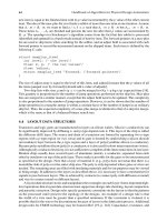
path exists. In the former case, retracing provides a shortest path between the source and the target
(Figure2.1).
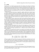
The input consists of a grid with blocked and nonblocked cells. The algorithm then goes through
three phases after the source and target have been chosen, and the source has been labeled with 0:
1. Wave propagation in which all unlabeled, nonblocked neighbors of labeled cells are labeled
one higher than in the preceding wave.
2. Retracing starts when the target has received a label and consists of repeatedly finding a
neighboring cell with a lower label, thus marking a shortest path between the source and
the target.
3. Label clearance prepares the grid for another search by adding the cells of the p ath just
found to the set of blocked cells and removing all labels.
The time needed to find a path is O(L
2
) if L is the length of the path. This makes it worst case
O(N
2
) on an N × N grid (and if each cell has to be part of the input, that is any cell can be initially
blocked, it is a linear-time algorithm). Its space complexity is also O(N
2
). These complexities were
13 13
13

13
13
13
13
13
13
13
13
13
13
13
13
13
13
13
1313
13
13
13
13
13
13
13
13
13
13
13
13
13
13

12
12
12
12
12
12
12
12
12
12
12
12
12
12
12
12
12
12
12
12
12
12
12
12
12
12
12
12
12
12

12
12
12
12
11
11
11
11
11
11
11
11
11
11
11
11
11
11
11
11
11
11
11
11
11
1111
11
11
11
11

11
11
11
11
11
11
10
10
10
10
10
10
10
10
10
10
10
10
10
10
10
10
10
10
10
10
10
10
10
10

10
10
10
10
10
10
9
9
9
9
9
9
9
9
9
9
9
9
9
9
9
9
9
9
9
9
9
9
9
9

9
9
T
8
8
8
88
8
8
8
8
8
8
8
8
8
8
8
8
8
8
8
8
8
7
7
7
7
7
7

7
7
77
7
7
7
7
7
7
7
6
6
6
6
6
6
6
6
6
6
6
6
6
5
5
5
5
5
5
5

55
5
5
4
4
4
4
4
4
4
4
4
3
3
3
3
3
3
3
2
2
2
2
2
1
1
1
S
FIGURE 2.1 Wave propagation and retracing. Waves are sets of grid cells with the same label. The source
S gets label 0. The target T gets the length of the shortest path as a label (if any). Retracing is not unique in

general.
Alpert/Handbook of Algorithms for Physical Design Automation AU7242_C002 Finals Page 11 24-9-2008 #4
Layout Synthesis: A Retrospective 11
soon seen as serious problems when applied to real-world cases. Some relief in memory use was
found in coding the labels: instead of labeling each explored cell with its distance to the source, it
suffices to record that number modulo 3, which works for any path search on an unweighted graph.
Here, however, the underlying structure is bipartite, and Akers [4] observed that wave fronts with a
label sequence in which a certain label bit is twice on and then twice off (i.e., 1, 1, 0, 0, 1, 1, 0, …)
suffice. Trivial speedup techniques were soon standard in maze running, mostly aimed at reducing
the wave size. Examples are designating the most off-center terminal as the source, starting waves
from both terminals, and limiting the search to a box slightly larger than the minimum containing
the terminals.
More significant techniques to reduce complexity were discovered in the second part of the
decade. There are two techniques that deserve a mention in retrospective. The first technique, line
probing, was discovered by David W. Hightower [5] and independently by Koichi Mikami and
Kinya Tabuchi [6]. It addressed both the memory and time aspects o f the router’s complexity. The
idea is for each so-called b ase point to investigate the perpendicular line segments that contain
the base point and extend those segments to the first obstacles on their way. The first base points
are the terminals and their lines are called trial lines of level 0 . Mikami and Tabuchi choose next as
base points all grid points on the lines thus generated. The trial lines of the next level are the line
segments perpendicular to the trial line containing their base point. The process is stopped when
lines originating from different terminals intersect. The algorithm guarantees a path if one exists
and it will have the lowest possible number of bends. This guarantee soon becomes very expensive,
because all possible trial lines of the deepest possible level have to be examined. Hightower therefore
traded it for more efficiency in the early stages by limiting the base points to the so-called escape
points, that is, only the closest grid point that allows extension beyond the obstacle that blocked the
trial line of the previous level. Line expansion, a combination of maze running and line probing,
came some ten years later [7], with the salient feature of p roducing a path whenever one existed,
though not necessarily with the minimum number of bends.
The essence of line probing is in working with line segments for representing the routing space

and paths. Intuitively, it saves memory and time, especially when the search space is not congested.
The complexity very much depends on the data structures maintained by the algorithm. The original
papers were vague ab out this, and it was not until th e 1980s that specialists in computational geometry
could come up with a rigorous analysis [8]. In practice, line probers were used for the first nets with
distant terminals. Once the routing space gets congested, more like a labyrinth where trial lines are
bound to be very short, a maze runner takes over.
The second technique worth mentioning is based o n the observation that from a graph theoretical
point of view,Lee’s router is just a breadth-first search that may take advantageofspecial features like
regularity and bipartiteness. Bu t significant speed advantage can be achieved by including a sense
of direction in the wave propagation phase, p referring cells closer to the target. Frank Rubin [9]
implements such an idea by sorting the cells in the wavefront with a key representing the grid
distance to the target. It shifts the character of the algorithm from breadth-first to d epth-first search.
This came c lose to what was developed simultan eously, but in the field of artificial intelligence:
the A
∗
algorithm [10]. Here the search is ordered by an optimistic estimate of the source–target
pathlength through the cell. The sum of the number of steps to reach that cell (exactly as in the
original paper of Lee) plus the grid distance to the target (as introduced by Rubin) is a satisfactory
estimate, because the result can never be more than that estimate. This means that it will find the
shortest route, while exploring the least number o f grid cells. See Chapter 23 for a more detailed
description of maze routing.
Lee’s concept combined with A
∗
is still the basis of modern industrial routers. But many more
issues than just the shortest two-pin net have to be considered. An extension to multiterminal nets is
easy (e.g., after connecting two pins, take th e cells on that route as the initial wavefront and find the
shortest path to another terminal, etc.), but it will not in general produce the shortest connecting tree
(for this the Steiner problem on a grid has to be solved, a well-known NP-hard problem, which is