Handbook of algorithms for physical design automation part 8 pps

Alpert/Handbook of Algorithms for Physical Design Automation AU7242_C003 Finals Page 52 29-9-2008 #25
52 Handbook of Algorithms for Physical Design Automation
26. S. Mutoh et al. 1-V power supply high-speed digital circuit technology with multithreshold voltage CMOS.
IEEE Journal of Solid-State Circuits, 30(8):847–854, August 1995.
27. D. Lee, D. Blaauw, and D. Sylvester. Static leakage reduction through simultaneous υ
t
/t
ox
and state assign-
ment. IEEE Transactions on Computer-Aided Design of Integrated Circuits and Systems, 24(7):1014–1029,
July 2005.
28. K. Kanda, K. Nose, H. Kawaguchi, and T. Sakurai. Design impact of positiv e temperature dependence on
drain current in sub-1-V CMOS VLSIs. IEEE Journal of Solid-State Circuits, 36(10):1559–1564, October
2001.
29. V. Gerousis. Design and modeling challenges for 90 nm and 50 nm. In Proceedings of the IEEE Custom
Inte grated Circuits Conference, San Jose, CA, pp. 353–360, 2003.
30. D. K. Schroder. Negative bias temperature instability: Road to cross in deep submicron silicon semicon-
ductor manufacturing. J ournal of Applied Physics, 94(1):1–18, July 2003.
31. M. A. Alam. A critical examination of the mechanics of dynamic NBTI for pMOSFETs. In IEEE
International Electronic D evices Meeting, Washington, D.C., pp. 14.4.1–14.4.4, 2003.
32. S. V. Kumar, C. H. Kim, and S. S. Sapatnekar. An analytical model for negative bias temperature instability
(NBTI). In Proceedings of the IEEE/ACM International Conference on Computer-Aided Design, San Jose,
CA, pp. 493–496, 2006.
33. A. M. Yassine, H. E. Nariman, M. McBride, M. Uzer, and K. R. Olasupo. Time dependent breakdown of
ultrathin gate oxide. IEEE Transactions on Electron Devices, 47(7):1416–1420, July 2000.
34. J. H. Lienhard and J. H. Lienhard. A Heat Transfer Textbook, 3rd edn. Phlogiston Press, Cambridge, MA,
2005.
35. Y. Cheng and S. M. Kang. A temperature-aware simulation environment for reliable ULSI chip design.
IEEE Transactions on Computer-Aided Design of Integrated Circuits and Syst ems, 19(10):1211–1220,
October 2000.
36. T. -Y. Wang and C. C. -P. Chen. 3-D thermal-ADI: A linear-time chip lev el transient thermal simulator. IEEE

Transactions on Computer-Aided Design of Integrated Circuits and Systems, 21(12):1434–1445, December
2002.
37. Y. Zhan, B. Goplen, and S. Sapatnekar. Electrothermal analysis and optimization techniques for nanoscale
integrated circuits. In Proceedings of the Asia/South Pacific Design Automation Conference, Yokohama,
Japan, pp. 219–222, 2006.
38. H. Qian, S. Nassif, and S. Sapatnekar. Random walks in a supply network. In Pr oceedings of the ACM/IEEE
Design Automation Conference, Anaheim, CA, pp. 93–98, 2003.
39. P. Li, L. T. P ileggi, M. Ashehi, and R. Chandra. IC thermal simulation and modeling via efficient multigrid-
based approaches. IEEE Transactions on Computer-Aided Design of Integrated Cir cuits and Systems,
25(9):1763–1776, September 2006.
40. S. Sapatnekar, Timing, Kluwer Academic Publishers, Boston, MA, 2004.
Alpert/Handbook of Algorithms for Physical Design Automation AU7242_S002 Finals Page 53 24-9-2008 #2
Part II
Foundations
Alpert/Handbook of Algorithms for Physical Design Automation AU7242_S002 Finals Page 54 24-9-2008 #3
Alpert/Handbook of Algorithms for Physical Design Automation AU7242_C004 Finals Page 55 24-9-2008 #2
4
Basic Data Structures
Dinesh P. Mehta and Hai Zhou
CONTENTS
4.1 Introduction 55
4.2 Input Data Structures 55
4.3 Data Structures Used during PD 57
4.3.1 Floorplanning Data Structures 57
4.3.2 Geometric Data Structures 57
4.3.2.1 Interval Trees 57
4.3.2.2 kd Trees 58
4.3.3 Spanning Graphs: A Global Routing Data Structure 59
4.3.4 Max-Plus Lists 60
4.4 Layout Data Structures 62

4.4.1 Corner Stitching 63
4.4.2 Quad Trees and Variants 65
4.4.2.1 Bisector List Quad Trees 66
4.4.2.2 kd Trees 67
4.4.2.3 Multiple Storage Quad Trees 67
4.4.2.4 Quad List Quad Trees 67
4.4.2.5 Bounded Quad Trees 68
4.4.2.6 HV Trees 68
4.4.2.7 Hinted Quad Trees 69
Acknowledgment 70
References 70
4.1 INTRODUCTION
Physical design automation may be viewed as the process of converting a circuit into a geometric
layout. We distinguish between three categories of data structures for the purpose of organizing this
chapter:
1. Data structures used to represent the input to physical design: the circuit or the netlist
2. Data structures used during the physical design process
3. Data structures used to represent the output of physical design: the layout
4.2 INPUT DATA STRUCTURES
A circuit consists of components and their interconnections. Each component contains logic that
implements some functionality. It also has pins (or terminals) with which it communicates with
other components. The entire circuit also needs to be able to communicate with the rest of the world
and does so through the use of external pins. An interconnection connects (or makes electrically
55
Alpert/Handbook of Algorithms for Physical Design Automation AU7242_C004 Finals Page 56 24-9-2008 #3
56 Handbook of Algorithms for Physical Design Automation
A
B
C
O

C1
C2
C3
C4
N2
N1
N3
N4
N5
N6
N7
Net 1: (A, C1.in1, C2.in1)
Net 2: (B, C1.in2, C3.in1)
Net 3: (C, C2.in2, C3.in2)
Net 4: (C1.out, C4.in1)
Net 5: (C2.out, C4.in2)
Net 6: (C3.out, C4.in3)
Net 7: (C4.out, O)
FIGURE 4.1 Circuit and its netlist.
equivalent) a set of two or more pins. These pins may be associated with the components or may be
external pins. Each intercon nection is called a net. The circuit is described by a list of all nets, the
netlist. Figure 4.1showsa simple example, where the components aresimple logic gates. Components
do not necessarily have to be logic gates. A componentcould be more complex.For example, it could
be a multiplier that was manually designed or designed by some other tool. The chip corresponding
to a circuit can itself be a component in a larger circuit.
The mathematical structure that comes closest to representing a circuit is the hypergraph. A
hypergraphconsists of a set of vertices and a set of hyperedges, where each hyperedgeconnects a set
of k ≥ 2 vertices. ( When k = 2 for each edge, the hypergraphreduces to the more familiar graph.) A
hypergraphapproximates a circuit in that each vertex is mapped to a component and each hyperedge
corresponds to a net. Even so, the hypergraph is not a complete representation of a circuit:

1. Components may have associated physical attributes. For example, if the component is a
rectangle, its height and width will be provided; locations of pins on the rectangle may also
be provided.
2. Nets have an associated direction, which p lay a role during routing. Consider Net 1 in
Figure 4.1 that interconnects th ree terminals. Pin A is the source of the signal and C1.in1
and C2.in1 are the sinks.
3. Nets connectpins, but hyperedgesconnectcomponents.Youcould fix this byhavingvertices
model pins rather than components, but then you lose the property that some pins are
associated with a single component. If this component is moved, all of its pins must move
with it.
The number of mathematical and algorithmic tools available for hypergraphs is small relative
to that for graphs. So, it is unlikely that there is much to be gained even if the hypergraph was
a complete representation. As a result, a netlist is sometimes represented by a graph. This is not
unreasonable because it turns out that the vast majority of nets are indeed two-terminal nets. There
is no well-defined way to convert a net with more than two terminals into one or more graph edges.
One approach is to add an edge between every pair of terminals in the net. A netlist converted into a
graph is often represented by a connectivity matrix. A matrix element in position [i][j] denotes the
number of nets that connect modules i and j.
∗
The netlist of Figure 4.1 is a complete description of a circuit. It may be read from a circuit
file, parsed and used to populate an internal data structure. This internal data structure is the start-
ing point of the physical design process. How should this internal data structure be organized? It
∗
This is actually a multigraph and not a graph because many edges are permitted between a pair of vertices.
Alpert/Handbook of Algorithms for Physical Design Automation AU7242_C004 Finals Page 57 24-9-2008 #4
BasicDataStructures 57
seems obvious that at a m inimum, the data structure should consist of a list of nets, where each net
object contains a list of pins. Should there also be a list of components where each component object
also contains a list of p ins? Should each component contain a list of nets that are incident on it? Is
it necessary to instantiate a pin object? If so, should it contain pointers to the component and net

to which it belongs? The answer to these questions depend on what kinds of queries will be posed
to the data structure by the particular physical design (PD) tool. One size does not fit all.
4.3 DATA STRUCTURES USED DURING PD
There are too many data structures in this category to describe in this chapter. Fortunately, the vast
majority of these are traditional data structures such as arrays, linked lists, search trees, hash tables,
and g raphs. We do not discuss these structures as they are typically covered in an undergraduate data
structures text (e.g., Ref. [1]). Graph algorithms are covered in Chapter 5. Below, we sample some
advanced data structures that have either been specifically d esigned with PD applications in mind or
have found widespread application in PD.
4.3.1 FLOORPLANNING DATA STRUCTURES
Several innovativedata structures (representations) have been developedfor floorplanning.We defer
a discussion of these data structures to the floorplanning section of the handbook, where they are
discussed in considerable detail (see Chapters 9 through 11).
4.3.2 GEOMETRIC DATA STRUCTURES
Each stage of physical design automation has a significant geometric aspect, with the possible
exception of partitioning that is more of a graph-theoretic problem. The computational geometry
literature [2] describes a number of geometric data structur es. The benefit of using geometric data
structures is that a query has a better time complexity than it would on a simple data structure such
as an array or a linked list. Implementing geometric data structures can be time consumin g, but they
may be found in algorithmic or geometric libraries [3,4]. A practitioner should weigh their benefits
against the simplicity of arrays and linkedlists. Examples of geometric data structuresinclude interval
trees, range trees, segment trees, kd trees, and priority search trees. Voronoi diagrams and Delaunay
triangulations may also be viewed as geometric data structures. Some of these structures can be
extended to higher dimensions although this comes at the cost of simplicity and time complexity.
Two or three dimensions are usually sufficient for physical design applications. These data structures
are often used in conjunction with the planesweep algorithm technique. Describing all of these data
structures is beyond the scope of this chapter. Instead, we pick two, the interval tree and kd tree, and
describe these briefly to give the reader a flavor of how they work.
4.3.2.1 Interval Trees
Most physical designs can be represented as a set o f axis-parallel rectangles. The boundaries of these

rectangles can be viewed as intervals. One common operation needed on these intervals is to find a
subset of them that intersect with a perpendicularline. Ifsuch a query only happens a limited number
of times, it can be efficiently processed by a sweep-line algorithm in O(n log n) time. However, when
such queries need to be done repeatedly, it is better to p reprocess the intervals and store them in a
data structure that can answer the queries more efficiently. The interval tree is a structure that can be
built in O(n log n) time and then answers the query in O(log n + k) time, where k is the number of
intervals intersecting the perpendicular line.
Even though an interval lies on a line that is a one-dimensional space, it is actually a two-
dimensional datum because it has two independent parameters. An interval starting at a and ending
at b is represented by [a, b]. It is not possible to have a total order over the set of intervals. The idea of
Alpert/Handbook of Algorithms for Physical Design Automation AU7242_C004 Finals Page 58 24-9-2008 #5
58 Handbook of Algorithms for Physical Design Automation
a
b
cd
ef
x
1
x
2
x
3
x
2
x
1
x
3
ee
bac cab

df fd
FIGURE 4.2 Set of intervals and its interval tree.
the interval tree is to partition the set o f intervals into three groups based on a given point x:intervals
to the left of the point L(x), intervals to the right of the point R(x), and intervals overlapping with
the point C(x). The subsets L(x) and R(x) of intervals can be recursively represented. The subset
C(x) also needs to be organized for the queries. Even though C(x) could include all the intervals in
the original set, organizing them is much simpler: they can be ordered both on their left points and
on their right points. If the query point q < x, only the left points of C(x) need to be checked in
increasing order; if q > x, only the right points of C(x) need to be checked in decreasing order. To
balance L(x) and R(x), thus to have a short tree, it is desired to use the median of all the endpoints
as x. Figure 4.2 shows an interval tree for a set of intervals, where the intervals in C(x) are organized
in two lists according to their left and right points.
The following result can be easily proved based on the above discussion.
Theorem 1 For a given set of n intervals, an interval tree can be constructed in O(n log n) time;
with it, a query on the intervals containing a given point can be answered in O (log n+k) time, where
k is the number of covering intervals.
Applications of interval trees may be found in Refs. [5–7].
4.3.2.2 kd Trees
The query facilitated bya kd tree can be viewed as the reverse ofth at b y an in tervaltree. In one dimen-
s
i
on, a set of points are given and a query by an interval wants to find all the points in it. If the queries
happen a limited number of times, they can be efficiently processed by linear scans of the points in
O(n) time. When queries needto be done frequently,a sorted array ora binary tree can be built by pre-
processing,and aquery can bedonein O(logn+k) timewhere k is thenumber ofpointson theinterval.
A kd tree is simply a n extension of this binary tree to higher dimension space. It first partitions
all the points into two groups of almost the same size along one dimension, and then recursively
partitions the groups along other dimensions. It follows the same order of dimensions for further
partitionings. Figure 4.3 shows a kd tree for a set of points on a plane (two-dimensional space)
0

1
2
4 5
63
7
0
1
2
3
4
5
6
7
a
b
c
d
e
f
g
h
i
j
a
8
8
b
e
cd
hf

jg
i
FIGURE 4.3 Set of points on the plane and its kd tree.
Alpert/Handbook of Algorithms for Physical Design Automation AU7242_C004 Finals Page 59 24-9-2008 #6
BasicDataStructures 59
Algorithm KdTreeQuery(v, R)
if
v
is a leaf
then output the point if it is in
R
else {
if
left
(
v
) is fully contained in
R
then output points in
left
(
v
)
else if
left
(v) intersects
R
then KdTreeQuery (
left
(

v
),
R
)
// similar code for
right
(
v
) omitted
}
FIGURE 4.4 R ange query algorithm on a kd tree.
with a horizontal partitioning followed by a vertical one. The algorithm for building a kd tree is
straightforward, based on recursive bipartitioning of the points along one dimension. Its runtime is
in O(n log n). Given an orthogonal range, a query on a kd tree will give all the points within the
range. The range query algorithm is just a simple extension of the interval query on binary trees and
it is described in Figure4.4.
Theorem 2 A kd tree for n points can be built in O(n log n) time; a query with an axis-parallel
range can be performed in O(n
1−1/d
+k) where d > 1 is the dimension and k is the number of points
within the range. In a two-dimensional plane, a query takes O(
√
n +k) time.
An application of the kd tree may be found in Ref. [8].
4.3.3 SPANNING GRAPHS: AGLOBAL ROUTING DATA STRUCTURE
Given a set of n points in a plane, a spanning tree is a set of edges that connects all n points and
contains no cycles. When each edge is weighted using some distance metric, the minimum spanning
tree is a spanning tree whose sum of edge weights is minimum. If Euclidean distance (L
2
)isused,

it is called the Euclidean minimum spanning tree; if rectilinear distance (L
1
) is used, it is called
the rectilinear minimum spanning tree (RMST). The RMST is often used as a starting point for
constructing a Steiner tree, which is used extensively in global routing (see Chapter 24).
The usual approach for constructing a minimum spanning tree is to first define a complete
weightedgraph on the set of pointsand then to constructa spanningtree on it, for example,by running
Kruskal’s algorithm (see Chapter 5).Given a set of points V, an undirectedgraph G = (V , E) is called
a spanning graph if it contains a minim um spanning tree. The cardinality of a grap h is its number
of edges. The complete graph has a cardinality of (n
2
), which is expensive. For the L
2
metric,
the Delaunay triangulation, a spanning graph of cardinality O(n), can be constructed in (n log n)
time. However, this approach does not work for the L
1
metric as the Delaunay triangulation may
be degenerate. Zhou et al. [9] describe a rectilinear spanning graph of cardinality O(n) that can be
constructedin O(n log n) time [9]. Its use in the construction ofa Steiner tree is described in Ref. [10].
We sketch the salient features of this data structure below.
Minimum spanning tree algorithms use two properties to infer the inclusion and exclusion of
edges in a minimum spanning tree:
1. Cut property states that an edge o f smallest weight crossing any partition of the vertex set
into two parts belongs to a minimum spanning tree.
2. Cycle property states that an edge with largest weight in any cycle in the graph can be safely
deleted.
Alpert/Handbook of Algorithms for Physical Design Automation AU7242_C004 Finals Page 60 24-9-2008 #7
60 Handbook of Algorithms for Physical Design Automation
R

1
R
2
R
3
R
4
R
5
R
6
R
7
R
8
s
s
p
q
(a) (b)
FIGURE 4.5 Octal partition of the plane.
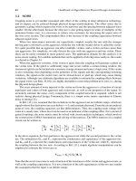
Define the octal partition of the plane with respect to s as the partition induced by the two
rectilinear lines and the two 45
◦
lines through s, as shown in Figure 4.5a. Here, each of the regions
R
1
through R
8
includes only one of its two bounding half line as shown in Figure 4.5b.

Lemma 1 Given a point s in the plane, each reg ion R
i
, 1 ≤ i ≤ 8, of the octal partition has the
property that for every pair of points p, q ∈ R
i
, pq < max(sp, sq).
Here spis the L
1
-distance between s and p. Consider the cycle on points s, p,andq and suppose
sp < sq. From the cycle property, edge sq can safely be excluded from the spanning graph.
This can be extended to excluding edges from s to all points in R
1
, except for the nearest one.
A property of the L
1
-metric is that the contour of equidistant points from s forms a line segment
in each region. In regions R
1
, R
2
, R
5
,andR
6
, these segments are captured by an equation of the form
x + y = c; in regions R
3
, R
4
, R

7
,andR
8
, they are described by the form x − y = c. This property is
used to devise a planesweep algorithm to construct the spanning graph. For each point s, we need to
find its nearest neighbor in each octant.We illustrate how to efficiently compute the nearest neighbor
in R
1
for each point. Other octants are similarly processed. For the R
1
octant, a sweep line is moved
along all points in increasing order of x +y. During the sweep, we maintain an active set consisting
of points whose nearest neighbors in R
1
are yet to be discovered. When a point p is processed, we
identify all points in the active set th at have p in their R
1
regions. Suppose s is such a point in the
active set. Because points are scanned in increasing x + y, p must be the nearest point to s in R
1
.
Therefore, we add edge sp to the spanning graph and delete s from the active set. After processing
these active points, we also add p to the active set. Each point is added and deleted at most once
from the active set. The runtime for the sweep is O(n log n). Each point s has an edge to its nearest
neighbor in each octant. This gives a spanning graph o f cardinality (n).
4.3.4 MAX-PLUS LISTS
Max-pluslists are applicableto slicing floorplans[11], technologymapping [12],and buffer insertion
[13] problems. Consider a list where each item consists of a pair of elements (m, p). Each item
represents a possible solution to an optimization problem that seeks to minimize both m and p (e.g.,
m and p could representthe height and width of a chip). Solutionj is said to be redundant with respect

to solution i if i.m ≤ j · m and i · p ≤ j · p because it is no better than i on either attribute. Consider
a list of three solutions: S
1
= (5, 4), S
2
= (4, 6),andS
3
= (5, 5). S
3
is redundant wrt S
1
. Neither S
1
nor S
2
is redundant wrt any of the other solutions. Redundant elements are discarded from the list.
Consider an ordered list A =[(A
1
· m, A
1
· p), , (A
q
· m, A
q
· p)] such that A
i
· m > A
j
· m ∧
A

i
· p < A
j
· p for any i < j. Such an ordering of solutions is always possible if redundant solutions
are not present in the list. Our example list of three elements above can be rewritten as [(5,4), (4,6)].
Alpert/Handbook of Algorithms for Physical Design Automation AU7242_C004 Finals Page 61 24-9-2008 #8
BasicDataStructures 61
These lists arise in the context of dynamic programming, which tries to find an optimal solution
to a problem by first finding optimal solutions to subproblems and then merging them to find an
optimal solution tothe larger problem.Each listrepresents possible optimal solutions toa subproblem.
Merging them gives us a list of possible optimal solutions to the bigger problem.
We next define th e list merge. Given two ordered lists A and B as defined above with q and r
elements, respectively, computeanother list C such that each elementc of C is obtainedby combining
an element a of A with an element b of B using the max-plus operation as follows:
c.m = max(a ·m, a ·m)
c.p = a · p +b · p
Redundant solutions are not permitted in C. Thus, C only contains the irredundant combinations
among the qr possible combinations of elements in A and B. Let the size of C be s.
To illustrate therationa le for the max-plus operation tocombine elements, considertwo rectangles
with dimensions h
1
× w
1
and h
2
× w
2
. Suppose one rectangle is stacked on top of the other and we
wish to determine the dimensions of the smallest bounding box that encloses both rectangles. The
height of this bounding box is the sum of the heights of the two rectangles while its width is the

maximum of the two rectangle widths; that is, the ma x plus operation. In buffer insertion, the two
quantities are delay (maximum operation) and downstream capacitance (plus operation).
Stockmeyer [11] proposed an algorithm to perform the list merge in time O(q + r).However,
when the merge tree is skewed, it takes r
2
time to combineall the lists even thoughthe total number of
items in C is r. Stockmeyer’s algorithm is inefficient when the two lists have very different lengths.
An extreme case is when a single item is being merged with a big list. In this case, the algorithm
reduces to a linear time search to find the location of an element in a sorted list. Balan ced binary
search trees [14] were used to represent each list so that a search can be done in O(log r) time. In
addition, to avoid updating the p values individually, the update was annotated on a node for the
rooted subtree. Shi’s algorithm is faster when the merge tree is skewed, with O(r logr) time relative
to Stockmeyer’s O(r
2
) time. However, Shi’s algorithm is complicated an d much slower when the
merge tree is balanced.
To summarize, the merge of two candidate lists using balanced binary search trees can only
speed up the merge of two candidate lists of very different lengths (unbalanced situation), but not
the merge of two candidate lists of similar lengths (balanced situation).
Figure 4.6 illustrates the best data structure for maintaining solutions in each of the two extreme
cases: the balanced situation requir es a linked list that can be viewed as a totally skewed tree; the
unbalanced situation requiresa balanced binarytree. However,most cases inreality are between these
extremes, where neither data structure is the best. The max-plus list is an efficient data structure for
the merge operation [15]. As shown in Figure 4.6, it can adapt to the structure of the merge tree: it
becomes a linked list in balanced situations and behaves like a balanced binary tree in unbalanced
situations. The merge algorithm based on max-plus list has the same asymptotic time complexity as
that used in Refs. [14,16] but is easier to implement and more efficient in practice [15].
The max-plus list is based on the skip list [17]. Because a max-plus list is similar to a linked list,
its merge operation is just a simple extension of Stockmeyer’s algorithm. During each iteration of
Stockmeyer’s algorithm, the current item with the max imal m value in one list is finished, and the

Linked list
(totally skewed tree)
Balanced binary tree
Max-plus list
Balanced situation Unbalanced situation
FIGURE 4.6 Flexibility of max-plus list.