Handbook of algorithms for physical design automation part 10 pps

Alpert/Handbook of Algorithms for Physical Design Automation AU7242_C004 Finals Page 72 24-9-2008 #19
Alpert/Handbook of Algorithms for Physical Design Automation AU7242_C005 Finals Page 73 23-9-2008 #2
5
Basic Algorithmic
Techniques
Vishal Khandelwal and Ankur Srivastava
CONTENTS
5.1 Basic ComplexityAnalysis 73
5.2 Greedy Algorithms 75
5.3 Dynamic Programming 76
5.4 Introduction to Graph Theory 77
5.4.1 Graph Traversal/Search 78
5.4.1.1 Breadth First Search 78
5.4.1.2 Depth First Search 78
5.4.1.3 Topological Ordering 79
5.4.2 Minimum Spanning Tree 79
5.4.2.1 Kruskal’s Algorithm 80
5.4.2.2 Prim’s Algorithm 80
5.4.3 Shortest Paths in Graphs 80
5.4.3.1 Dijkstra’s Algorithm 81
5.4.3.2 Bellman Ford Algorithm 81
5.5 Network Flow Methods 82
5.6 Theory of NP-Completeness 84
5.7 Computational Geometry 85
5.7.1 Convex Hull 85
5.7.2 Voronoi Diagrams and Delaunay Triangulation . 86
5.8 Simulated Annealing 86
References 87
This chapter provides a brief overview of some commonly used general concepts and algorithmic
techniques. The chapter begins by discussing ways of analyzing the complexity of algorithms, fol-
lowed by general algorithmic concepts like greedy algorithms and dynamic programming. This is

followed by a comprehensive discussion on graph algorithms including network flow techniques.
This is followed by discussions on NP completeness and computational geometry. The chapter ends
with the description of the technique of simulated annealing.
5.1 BASIC COMPLEXITY ANALYSIS
An algorithm is essentially a sequence of simple steps used to solve a complex problem. An algorithm
is considered good if its overall runtime is small and the rate at which this runtime increases with
the problem size is small. Typically, this runtime complexity is analytically measured/modeled as a
function of the total number of elements in the input problem. To make this analysis simpler, several
notations and conventions have been developed.
73
Alpert/Handbook of Algorithms for Physical Design Automation AU7242_C005 Finals Page 74 23-9-2008 #3
74 Handbook of Algorithms for Physical Design Automation
c2h(n)
c1h(n)
f(n)
n
n
0
f(n)
n
0
ch(n)
f(n)
n
n
0
ch(n)
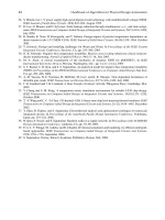
O -notation
Ω-notationΘ-notation
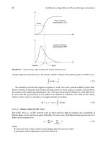
FIGURE 5.1 Complexity analysis.

-Notation
For a function h(n), [h(n)] represents the set of all functions that satisfy the following:
[h(n)]=
{
f (n): there exist positive constants c1andc2andann
0
such that
0 ≤ c 1h(n) ≤ f (n) ≤ c2h(n) ∀ n ≥ n
0
}
Conceptually, the set of functions f (n) are sandwiched between c1h(n) and c2h(n). In such scenarios,
h(n) is said to be the asymptotically tight bound (see Figure 5.1) for f (n). Therefore, if an algorithm
has a complexity of f (n) (takes f (n) steps to execute), then its complexity could be classified as
[h(n)].
O-Notation
For a function h(n), O[h(n)] represents a set of functions that satisfy the following:
O[h(n)]=
{
f (n): there exist positive constants c and an n
0
such that
0 ≤ f(n) ≤ ch(n) ∀ n ≥ n
0
}
The O-notation represents an upper bound (see Figure 5.1) for the set of functions f (n). Therefore,
an algorithm with complexity f (n) could be classified as an algorithm with complexity O[h(n)].
-Notation
For a function h(n), [h(n)] represents a set of functions that satisfy the following:
[h(n)]=
{

f (n): there exist positive constants c and an n
0
such that
0 ≤ ch(n) ≤ f (n) ∀ n ≥ n
0
}
The -notation represents a lower bound (see Figure 5.1) for the set of functions f (n).
E
XAMPLE
Analysis of the Complexity of Sort
Sort (Array:A, size:N):
last = N
While last >= 1
Alpert/Handbook of Algorithms for Physical Design Automation AU7242_C005 Finals Page 75 23-9-2008 #4
Basic Algorithmic Techniques 75
max = A[1]
max-location = 1
For i = 1 to last
If (A[i] > max)
max = A[i]
max-location = i
temp = A[max-location]
A[max-location] = A[last]
A[last] = temp
last = last − 1
Return A
The outer while loop runs N times. For the first time the inner loop runs N times, followed
by N − 1andthenN −2, etc. So the total number of iterations in this alg orithm become N + N −
1 +N −2 +···+1 = N(N +1)/2.
Now it can be seen that th e algorithmic complexity of sort, f (N) = N(N + 1)/2isO(N

2
) and
also (N
2
).
5.2 GREEDY ALGORITHMS
An algorithm is defined as a sequence of simple steps that solves a more complicated problem. At
each step, the algorithm makes a decision from a set of choices. Greedy algorithms [1] have the
property of making a choice that looks the best at that time. This may or may not guarantee the
optimality of the final solution. The key advantage of greedy algorithms is simplicity. In this section,
we will discuss thebasic properties that a problemmust have forgreedy strategies to yield the optimal
solution.If we can demonstrate the following properties in a problem,then greedy methodswill yield
the optimal solution:
1. Problem can be modeled as a combination of a greedy choice and a smaller subproblem.
2. There exists an optimal solution to the problem in which the greedy choice has been made.
3. Combination of the optimal solution to the subproblem and the greedy choice results in the
optimal solution to the overall problem.
E
XAMPLE
Fractional Knapsack Problem
Given a knapsack o f a certain size W and n items, with the ith item having a value of v
i
and a quantity
of w
i
. We would like to fill the knapsack with the maximum valued goods.
The algorithm is as follows:
1. Sort the items in decreasing order of v
i
/w

i
.
2. Start f rom t he first item in t he list and pick as much as you can.
3. If space still left, then go to the next item and repeat.
Note that we select as much as possible of the most valuable item (largest v
i
/w
i
). This is a greedy step.
The remaining space in the knapsack is filled by the remaining items. This constitutes the subproblem.
It can be shown that the above three properties hold for the fractional knapsack problem and therefore it
is solvable optimally using greedy strategies.
There are many problems (including the 0–1 generalization of the knapsack problem where we are
forced to choose the entire item or none at all) where a greedy scheme cannot guarantee optimality. In
Alpert/Handbook of Algorithms for Physical Design Automation AU7242_C005 Finals Page 76 23-9-2008 #5
76 Handbook of Algorithms for Physical Design Automation
such scenarios, greedy schemes are usually employed as heuristics resulting in quick but good solutions
to the problem, although not provably optimal.
5.3 DYNAMIC PROGRAMMING
The technique of dynamic programming (DP) [1] essentially is a way of utilizing the availability
of cheap memory to improve the runtime of algorithms. This technique was invented by Richard
Bellmanin 1953. Before we go into thedetails ofthis technique,let usdiscuss the followingsequence
of steps for solving a problem:
1. Break the problem into smaller subproblems.
2. Solve the smaller subproblems optimally.
3. Combine the optimal solutions to the smaller subproblems to get a solution to the original
problem.
Now the term optimal substructure means that the optimal solution to the subproblems can be
used to generate the optimal solution to the overall problem. If indeed this is true then the above-
mentioned sequence of steps for solving a problem must generate the optimal solution to the overall

problem. DP also generates the optimal solution using the same principle. Let us illustrate the DP
philosophy using an example.
E
XAMPLE
Generation of the Nth Fibonacci Number
Solution
A simple way of gener ating the Nth Fibonacci number could be as follows:
FIBONACCI(N)
If N = 0or1
then return N
Else
return FIBONACCI(N −1) + FIBONACCI(N −2)
Note that this problem demonstrates optimal substructure because the optimal solution to the
problem of size N can be generated by the optimal solution for subproblem of size N −1andN −2.
The complexity of this algorithm could be analyzed as follows. Let T(N) represent the complexity
of optimally solving a problem of size N.So
T(N) = T(N − 1) +T(N − 2) for N > 1
It could be shown that T (N) is an exponential function of N, which clearly is impractical for
large problems. Nonetheless, from close inspection, we find that to solve the subproblem of size
N − 1, we will inevitably solve a subproblem of size N − 2. This property is called overlapping
subproblems. Existence of overlapping subproblems could be utilized to improve the complexity of
the above algorithm. Basically, every time a subproblem of a certain size is encountered for the first
time, its optimal solution could be stored. Next time, if the optimal solution to this subproblem is
needed, it could simply be accessed from memory. Using such techniques, a modified algorithm for
Fibonacci numbers is as follows:
MODIFIED FIBONACCI(N)
For i = 1toN
M[i] =−1
Function Fib(N)
Alpert/Handbook of Algorithms for Physical Design Automation AU7242_C005 Finals Page 77 23-9-2008 #6

Basic Algorithmic Techniques 77
If M[N] ! =−1
M[N] = Fib(N −1) + Fib(N −2)
return M[N]
In this algorithm, the array M stores the optimal solution (Fibonacci values). Whenever the
solution of a subproblem is needed, it could be simply read from this array without having to
perform the whole computation again from scratch. This technique is called memoization. It could
be seen that the complexity of this algorithm is no longer exponential.
Although the Fibonacci example is not an optimization p roblem, it illustrates the concept behind
DP quite well. DP is essentially a divide-and-conquer approach in which larger complex problems
are subdivided in simpler subproblems. The existence of the optimal substructure property ensures
that optimality of the overall problem will be maintained. Furthermore, overlapping subproblems
could be stored in memory (memoization) for improving the runtime complexity of the algorithm.
DP-based approaches for a given problem could be developed as follows:
1. Express the overall problem in the form of subproblems.
2. Investigate if the optimal substructure property holds.
3. Investigate the existence of overlapping subproblems.
4. Develop a memoization-based approach in which the solutions to overlapping subproblems
are stored in memory, hence improving the computational complexity.
Several physical design/synthesis problems including buffer insertion for wiring trees and
technology mapping could be solved optimally using DP [5].
5.4 INTRODUCTION TO GRAPH THEORY
Graph theory [1,2] is believed to have begun in the year 1736 with the publication of the solution to
the Konigsberg bridge problem, developed by Euler. A graph is characterized by G = (V, E),where
V is the set of vertices and E is the set of edges between them (see Figure 5.2). These edges could
either be directed (leading to a directed graph) or undirected (undirected graph). Graphs provide an
excellent way to abstract various problems in physical synthesis and design. Combinational circuits
are typically modeled as directed acyclic graphs and placement netlists are also modeled as graphs.
Definition 1 Path: A sequence of vertices and edges in which no vertex is repeated.
Definition 2 Cycle: A sequence of vertices v

0
, v
1
, v
2
, , v
n
where v
n
= v
0
and all other vertices
are different.
TreePath Cycle
FIGURE 5.2 Examples of graphs.
Alpert/Handbook of Algorithms for Physical Design Automation AU7242_C005 Finals Page 78 23-9-2008 #7
78 Handbook of Algorithms for Physical Design Automation
5.4.1 GRAPH TRAVERSAL/SEARCH
Searching a graph is the process of hopping from one vertex to the other in search for the appropriate
vertex or edge. Graph search is used extensively in physical synthesis and design problems when
a gate of a specific characteristic is being searched. It also finds widespread application in timing
analysis. Two schemes for searching on a graph have been developed
5.4.1.1 Breadth First Search
Given a graph G = (V, E) and asource vertexs,breadth first search (BFS) systematically investigates
all the vertices that can be reached from s. The algorithm is outlin ed below:
BFS(G(V,E),s)
For each vertex u ∈ V −{s}
Status[u] = untouched
Distance[u] =∞
Distance[s] = 0

QUEUE ={s}
While QUEUE! = NULL
u = FRONT(QUEUE) /
∗
The function FRONT returns the front
of a queue
∗
/
For each vertex v that can be directly reached from u
If Status[v] = untouched
Status[v] = touched
Distance[v] = Distance[u] + 1
ENQUEUE(QUEUE, v)
DEQUEUE(QUEUE) /
∗
Remove the Front Vertex from the Queue
∗
/
Status[u] = Finished
In this algorithm, the frontier between the discovered and undiscovered vertices proceeds like
a wavefront. Starting from the source, all vertices immediately adjacent to it are investigated. This
is followed by investigation o f all vertices adjacent to these and so on. This algorithm finds the
minimum number o f edges between the source s and the vertices that are reachable from s (this
information gets stored in the array Distance). If a vertex cannot be reached then its distance from
the source is in finity.
5.4.1.2 Depth First Search
Unlike BFS that proceeds as a wavefront, depth first search (DFS) investigates deeper in the graph
till it cannot go any further. At this point, it backtracks to the nearest vertex and investigates its
neighbors once again in a depth first manner. This process continues till no further vertices can be
explored. The algorithm is outlined below:

DFS(G(V,E)) Touch-DFS(u)
For each vertex u Status[u] = touched
Status[u] = untouched Time = Time + 1
Time = 0 Starting-Time[u] = Time
For each vertex u For each v that can be reached from u
If Status[u] = untouched If Status[v] = untouched
Alpert/Handbook of Algorithms for Physical Design Automation AU7242_C005 Finals Page 79 23-9-2008 #8
Basic Algorithmic Techniques 79
Touch-DFS(u) Touch-DFS(v)
Status[u] = finished
Time = Time + 1
Finishing-Time[u] = Time
As indicated in the algorithm above, we start with a vertex and investigate deeper into the
neighborhood till we cannot go any further. At this point, we go one level above to the p revious
vertex and investigate deep into the graph once again. A vertex is deemed finished if all the vertices
adjacent to it have been touched in a depth first manner. Note that Starting-Time and Finishing-Time,
respectively, indicate the time stamp at which we begin investigating a vertex and at which we have
investigated its entire neighborhood.
The runtime complexity of both BFS and DFS is O(|V|+|E|).
5.4.1.3 Topological Ordering
Definition 3 Directed Acyclic Graph (DAG): A directed graph G = (V, E) in which there are no
directed cycles.
Directed acyclic graphs can be used to model most combinational circuits and therefore are
particularly important for VLSI computer-aided design (CAD). Topological ordering in DAGs is an
ordering v
0
, , v
n
of all vertices in V such that for a given vertex v
i

, all the vertices in V that have a
path either directly or indirectly to v
i
must come before v
i
in this ordering.
Topological ordering can be generated using DFS by sorting the nodes in decreasing order of
their finishing times.
5.4.2 MINIMUM SPANNING TREE
Let us suppose we have an undirected graph G = (V, E) where each edge (u, v) has a weight w(u, v).
A spanning tree on such a graph is defined as follows:
Definition 4 Spanning tree: A spanning tree of a graph G = (V, E) is a subgraph G

= (V, E

),
which has the same vertices as G and the edges E

⊆ E such that G

forms a tree.
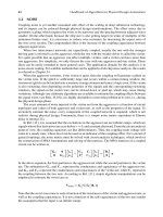
A minimum spanning tree (MST) of a graph G is a spanning tree with th e minimum total
weight (of all edges) among all possible spanning trees of G (see Figure 5.3). There are two popular
algorithms for finding the MST of a graph: Kruskal’s algorithm and Prim’s algorithm.
Initial graph MST
4
15
3
25
2

1
FIGURE 5.3 Minimum spanning tree.
Alpert/Handbook of Algorithms for Physical Design Automation AU7242_C005 Finals Page 80 23-9-2008 #9
80 Handbook of Algorithms for Physical Design Automation
5.4.2.1 Kruskal’s Algorithm
Kruskal’s algorithm proceeds by starting with a set of disconnected trees (a forest) of vertices in G
and merges them in such a way that we eventually get the MST of G. The algorithm is as follows:
Kruskal(G =(V,E))
Each node in G represents a trivial Tree.
Sort all edges in E in non-decreasing order of weights
For each edge (u,v) ∈ E in the non-decreasing order
If u and v are in separate trees
Merge the two trees into one by connecting them
through the edge (u,v)
The algorithm starts by assigning all nodes to separate trees. Then it traverses the edges in
nondecreasing order of their weights. If an edge merges two separate trees then it is used to create a
larger tree otherwise it is discarded. The algorithm terminates after generating the MST.
5.4.2.2 Prim’s Algorithm
Unlike Kruskal’s algor ithm, that maintains multiple trees and merges them iteratively, Prim’s algo-
rithm has only one tree and merges more vertices in this tr ee till the MST is created. The algorithm
is outlined as follows:
Prim(G =(V,E))
Start with any vertex in V and assign it to a Tree T
While there exist vertices in G not in T
Find a vertex in G-T which is closest to T
Expand T by including this vertex
MSTs are used extensively in physical design to predict the wirelengh of interconnects when the
placement information is available and routing is not known.
5.4.3 SHORTEST PATHS IN GRAPHS
The problem of shortest paths in graphs has several important practical applications. Given a graph

G = (V, E) (directed or undirected) and edge weights, try to find the shortest weighted path from
a given source s to all other vertices (single-source shortest path problem) or between all pair of
vertices. The overall weight of a path is simply the sum of all the edge weights on it.
Let us start the discussion with the single-source shortest path problem. Given a source s,we
would like to find the shortest p ath to all other vertices in the graph. Definition of a shortest path
between two vertices becomes ambiguous when there exists a negative weight cycle between the
source and the destination. We can simply find a shorter route by indefinitely going around this
negative cycle (and therefore reducing the overall path weight). We describe two algorithms for
finding the shortest paths: Dijkstra’s algorithm and Bellman Ford algorithm. Dijkstra’s algorithm
assumes all the edge weights are positive and therefore there are no negative weighted cycles either.
On the other hand, Bellman Ford algorithm can handle negative weighted edges and also detect the
existence of negative weighted cycles (a case where shortest path is not defined).
Alpert/Handbook of Algorithms for Physical Design Automation AU7242_C005 Finals Page 81 23-9-2008 #10
Basic Algorithmic Techniques 81
5.4.3.1 Dijkstra’s Algorithm
This algorithm takes a weighted graph G with positive edge weights, a source vertex, and generates
the shortest weighted path solution. It initializes two sets S and S

.ThesetS consists of all vertices in
G whose shortest path from s has been calculated and the set S

consists of all the remaining vertices.
Initially, S ={s} and S

= V −{s}. We also initialize a label array L, which stores the labeling for
the vertices. The moment a vertex u is included in the set S, its labeling L[u] is exactly the weight of
the shortest p ath between s and u. Initially, L[s]=0andL[u]=∞∀u ∈ V −{s}. In the next step,
the labels of all the vertices v in S

, which are adjacent to a vertex u in S are updated as follows. If

L[u]+weight(u, v) ≤ L[v] then L[v]=L[u]+weight(u,v). After updating all the labels, the vertex
in S

that has the smallest label is chosen and moved to the set S. At this point, the label of this node
corresponds to the weight of the shortest path from s. These sequence of steps are continued till S

is null. The algorithm is formally outlined below:
Dijkstra(G =(V,E))
S ={s},S

= V −{s}
L[s] = 0, L[u] =∞ ∀ u ∈ V −{s}
L[u] = weight[su] ∀ u adjacent to s
While S

! = NULL
Find Minimum L[u] ∀ uinS

S = SU {u}
S

= S

−{u}
For each v in S

that is adjacent to u
If L[v] ≥ L[u] + weight(uv)
L[v] = L[u] + weight(uv)
It could be seen that this is a greedy algorithm because at each step a greedy choice is executed

(the vertex with the smallest labeling is chosen). This greedy algorithm indeed results in the optimal
solution.
5.4.3.2 Bellman Ford Algorithm
Dijkstra’s algorithm cannot handle edge weights that are negative. Bellman Ford algorithm not only
handles negative edge weights but also detects the existence of negative weighted cycles (that are
reachable from the source s). The algorithm is iter ative in nature. Once again it has a label array L.
L[s] is initializes to 0 and infinity for all other vertices. The algorithm is outlined below:
Bellman Ford (G =(V,E))
L[s] = 0, L[u] =∞∀u ∈ V −{s}
For i = 1 to Number of Vertices
For each edge (u,v) ∈ E
If L[v] ≥ L[u] + weight(uv)
L[v] = L[u] + weight(uv)
The algorithm is quite self-explanatory. It could be proved that if there are no negative
weighted cycles reachable from s then the array L has the shortest path to each vertex in the graph.
Detection of negative weighted cycles (reachable from s) can be done by the following simple
procedure:
Negative Cycle Detection
Let L be the labeling of all nodes after application
of Bellman Ford