Handbook of algorithms for physical design automation part 14 ppsx

Alpert/Handbook of Algorithms for Physical Design Automation AU7242_C007 Finals Page 112 24-9-2008 #5
112 Handbook of Algorithms for Physical Design Automation
For example, a net consisting of four vertices is represented by an equivalent six-edge complete
graph. To cut off one vertex from the rest requires cutting three edges, so the weight should be 1/3
(for a total edge weight of 1). However, to cut off two vertices from the rest requires cutting four
edges (each with weight 1/4). Because some of the edges assigned weights of 1/3 and 1/4 may be
the same, this weighting scheme is inconsistent.
Lengauer [Len90] proves that no matter what weighting scheme is selected, there will always
exist an exact graph bipartition with a deviation of (
√
|e|) from the cost of cutting a single net.
Additionally, Ihler et al. [IWW93] conjecture that a clique graph model is the best in terms of
deviation from the true cost of cutting one net.
In the generic cliq ue model, a net on |e| vertices induces a complete graph where each edge has
weight
w
i
=
1
|e|−1
This weighting scheme arises from linear placements into fixed slots separated by a unit distance.
The denominato r indicates the minimum total wirelength used to connect the |e| ver tices. Vannelli
and Hadley [VH90] propose the following metric that guarantees the weight of edges cut under a
k-way partitioning has an upper bound of 1.
w
i
=
1

|e|
k


|e|
k

Huang [HK97] proposes a weight of
w
i
=
4
|e|(|e|−1)
that distributes the weight of one net evenly across two edges and gives an expected cut weight of 1.
The following weighting scheme distributes the edge weight evenly across |e|−1 edges:
w
i
=
2
|e|
In Ref. [AY95], the authors use a variant of Huang’s metric:
w
i
=
4
|e|(|e|−1)
2
|e|
− 2
2
|e|
7.1.2 PARTITIONING AND CLUSTERING METRICS
In this section, we give some definitions relevant to hypergraph partitioning and use them to describe

metrics used in hypergraph partitioning.
Definition 3 Given a hypergraph, G(V, E), nets that have vertices in multiple blocks belong to
the cutset, E
c
, of the hypergraph. Given k blocks, the cutset between the ith pair of blocks where
i = 1 ···

k
2

is denoted by E
c
i
.
Definition 4 A partition, f (V , k), o f the set of vertices, V , into k blocks, {C
1
, , C
k
} is given by
C
1
∪ C
2
∪···∪C
k
= VwhereC
i
∩ C
j
=∅and α|V|≤|C

i
|≤β|V | for 1 ≤ i < j ≤ k and
0 ≤ α, β ≤ 1.
Alpert/Handbook of Algorithms for Physical Design Automation AU7242_C007 Finals Page 113 24-9-2008 #6
Partitioning and Clustering 113
Definition 5 The weight of the ith block is denoted by w(C
i
). Usually, it is equal to the number
of vertices in the ith block, |C
i
|
Definition 6 Given a clustering solution {C
1
, C
2
, , C
k
},whereC
i
indicates a group of vertices,
construct a clustered hypergraph H

(V

, E

) such that for every e ∈ E, there is a hyperedge e

∈ E


with e

={C|∃υ ∈ e ∩C}.
Mincut partitioning: This metric counts the number of nets running between pairs of blocks
min f (V, k) =

k
i=1
|E
c
i
|
s.t. α|V |≤w(C
i
) ≤ β|V|
For example,if a net spans three blocks then it would be counted three times in the objective [Alp96].
A slightly different objective is one that counts the number of entire nets that are cut (this is formally
called the netcut). These objectives are identical if the number of blocks is two. Typically, α = 0.45
and β = 0.55 for bipartitioning. For k-way partitioning, some authors favor the following constraints:
|V |
αk
≤ w(C
i
) ≤
α|V |
k
where α>1 [KK99].
Min-ratiocut bipartitioning: The ratiocut metric, r
c
, is u sed in Refs. [WC91], [RDJ94] and others

as a way of incorporating balance constraints into the objective. The objective is
min f (V ,2) = r
c
=
|E
c
|
w(C
1
)w(C
2
)
where the numerator indicates the netcut. Fo r a given netcut, this metric is minimized when the two
blocks are of equal size. However, as Alpert and Kahng [AK95] pointout, the weakness in this metric
is that r
c
is very sensitive to change in |E
c
| and relatively unaffected by changes in w(C
1
) or w(C
2
).
Thus, given a small enough netcut, it is possible to obtain a minimal ratio cut even if the block sizes
are uneven.
In the analytic bipartitioning technique described in Ref. [RDJ94], vertices are assigned to
positions along the x-axis, simultaneously. Block assignments are then derived from the coordinates
in some fashion. Thus, it is not possible to move individual vertices from one block to another as
is the case with iterative-based partitio ners. Consequently, vertices may b e assigned positions along
the x-axis that do not satisfy even fairly loose balance constraints in which a block is allowed to h ave

between 45 and 55 percent of the cells (or total cell area).
Min-ratiocut k-way partitioning: Chan et al. [CSZ94] generalize the ratiocut metric for k blocks to
k

i=1

|E
c
i
|
w(C
i
)

≤
k

i=1
λ
i
where λ
i
is the ith smallest eigenvalue of the Laplacian matrix of G(V , E).
Scaled cost: Another metric that combines the usual minimum cut objective with block size
constraints is
f (V , k) =
1
|V |(k − 1)
k


i=1
|E
c
i
|
w(C
i
)
This metric is used in Refs. [AK93,AK94,AK96, KK98,AKY99].
Alpert/Handbook of Algorithms for Physical Design Automation AU7242_C007 Finals Page 114 24-9-2008 #7
114 Handbook of Algorithms for Physical Design Automation
C
e
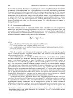
FIGURE 7.3 Absorption metric.
Absorption: The absorption metric measures the sum of nets, as a fraction, that are absorbed by
blocks [SS95].
max
k

i=1

{e∈E|e∩C
i
=∅}
|e ∩C
i
|−1
|e|−1
At the two extremes, nets that have one vertex in a block C add 0 to the absorption metric; nets that
have all vertices in a block C add 1 to the absorption metric. In Figure 7.3, |e ∩ C|=2,

|e∩C|−1
|e|−1
=
1
3
.
In addition to the usual balance constraints, partitio ning formulations may include constraints for
vertices that are assigned to a specific block. The presence of fixed terminals adds some convexity
to this otherwise highly nonconvex problem, making it computationally less expensive [EAV99]. In
Ref. [ACKM00], the authors point out that the presence of fixed vertices makes the problem trivial
in the sense that only one or two passes of an iterative improvement engine are required to approach
a good solution.
7.2 MOVE-BASED PARTITIONING METHODS
In this section, we will outline the most significant developments in the field of iterative improvement-
based partitioning. Iterative improvement forms the basis of multilevelpartitioning, which represents
the state of the art as far as partitioning is concerned.
7.2.1 KERNIGHAN–LIN HEURISTIC
Kernighan and Lin’s work was the earliest attempt at moving away from exhaustive search in
determining the optimal netcut subject to balance constraints. In Ref. [KL70], they propose a
O(|V |
2
log |V |) heuristic for graph bipartitioning based on exchanging pairs of vertices with the
highest gain between two blocks, C
1
and C
2
. They define the gain of a pair of vertices as the number
of edges by which the netcut decreases if vertices x and y are exchanged between blocks. Assuming
a
ij

are entries of a graph adjacency matrix, the gain is given by the formula
g(v
x
, v
y
) =
⎛
⎝

v
j
∈C
1
a
xj
−

v
j
∈C
1
a
xj
⎞
⎠
+
⎛
⎝

v

j
∈C
2
a
yj
−

v
j
∈C
2
a
yj
⎞
⎠
− 2a
xy
The terms in parentheses count the number of vertices that have edges entirely within one block
minus the number of vertices that have edges connecting vertices in the complementary block.
Alpert/Handbook of Algorithms for Physical Design Automation AU7242_C007 Finals Page 115 24-9-2008 #8
Partitioning and Clustering 115
TABLE 7.1
Gain Computations
Previous State Next State Gain
AB|AB
A
|+|OAB
A
|−|IA|−|OA|
BA|IAB

A
|+|OAB
A
|−|IA|−|OA|
The procedure works as follows: vertices are initially divided into two sets, C
1
and C
2
. A gain is
computed for all pairs of vertices (v
i
, v
j
) with v
i
∈ C
1
and v
j
∈ C
2
; the pair of vertices,(v
x
, v
y
), with the
highest gain is selected for exchange;v
x
and v
y

are then removedfromthe list of exchangecandidates.
The gains for all pairs of vertices, v
i
∈ (C
1
−{v
x
}) and v
j
∈ (C
2
−{v
y
}), are recomputed and the
pairing of vertices with the highest gain are exchanged. The process continues until g(v
x
, v
y
) = 0,
at which point, the algorithm will have found a local minimum. The algorithm can be repeated to
improve upon the current local minimum. Kernighan and Lin observe that two to four passes are
necessary to obtain a locally optimal solution.
In Ref.[SK72], Schweikertand Kernighan introduceamodelthat dealswith hypergraphsdirectly.
They point out that the major flaw of the (clique) graph model is that it exaggerates the importance
of nets with more than two connections. After bipartitioning, vertices connecting large nets tend to
end up in the same block, whereas vertices connected to two point nets end up in different blocks.
They combine their hypergraph model in the Kernighan–Lin partitioning heuristic and obtain much
better results on circuit partitioning problems.
7.2.2 FIDUCCIA–MATTHEYSES HEURISTIC
The Fiduccia–Mattheyses (FM) [FM82] meth od is a linear-time, [O(|P|)] per pass, hypergraph

bipartitioning heuristic. Its impressive runtime is due to a clever way of determining which vertex to
move based on its gain and to an efficient data structure called a bucket list.
Borrowing the terminology and notation from Ref. [KN91], a critical net is one that is connected
to a single vertex in one of the blocks (so that the removal of that vertex removes the net from that
block). A net state is a combination of subnetworks that contain a net as well as the subnetworks in
which the net is critical. Let A indicate that a net is entirely within block A;letA
A
indicate that a net
in block A is critical to block A.LettheprefixI or O indicate that the net is an input or output to the
vertex, thus IAB
A
indicates the input net has vertices in blocks A and B but that is critical to block A.
The gain equations are computed with respect to vertices and are given in Table 7.1.
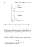
In Figure 7.4, if we move vertex u from A to B, the gain is co mputed in the following way.
|AB
A
|=2 becau se nets 1 and 2 are critical to A, |OAB
A
|=2 refers to nets 1 and 2 as well, |IA|=3
AB
Net 1
Net 2
v
u
FIGURE 7.4 Example of gain computations.
Alpert/Handbook of Algorithms for Physical Design Automation AU7242_C007 Finals Page 116 24-9-2008 #9
116 Handbook of Algorithms for Physical Design Automation
because there are three inputs to u in A,and|OA|=2 because there are two outputs to u in A.The
gain is given by |AB
A

|+|OAB
A
|−|IA|−|OA|=2 +2 −3 −2 =−1, which implies moving vertex
u will result in the netcut increasing by 1. On the other hand, moving vertex v from B to A imp lies
|IAB
A
|=1 because v has one input that is critical to A, |OAB
A
|=0 because v has no outputs critical
to A, |IA|=0 because v has no inputs in A,and|OA|=0 b ecause v has no outputs in A, for a total
gain of 1.
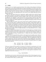
The gains are maintained in a [−|P|
max
···|P|
max
]bucket array whose ith entry contains a doubly
linked list of f ree vertices with gains currently equal to i . The maximum gain, |P|
max
, is obtained
when a vertex of degree |P|
max
(i.e., a vertex that is incident on |P|
max
nets) is moved across the block
boundary and all of its incident nets are removed from the cutset (Figure7.5).
The free vertices in the bucket list are linked to vertices in the main vertex array so that during a
gain update, vertices are removed from the bucket list in constant time (per vertex). Superior results
are obtained if vertices are removed and inserted from the bucket list using a last-in-first-out (LIFO)
scheme (over first-in-first-out [FIFO] or random schemes) [HHK97]. The authors of Ref. [HHK97]
speculate that a LIFO implementation is better because vertices that naturally block together will

tend to be listed seq uentially in the netlist. Car e must be exercised to compute gains cor rectly for
situations where a cell has two inputs on the same net.
7.2.3 IMPROVEMENTS ON THE F IDUCCIA–MATTHEYSES HEURISTIC
This section discusses a few noteworthy improvements to the orig inal FM implementation that have
helped the acceptance of FM as the most popular partitioning technique.
The first improvement to FM is Krishnamurthy’s look-ahead scheme [Kri84], in which a vertex
belonging to a multivertex net, which is in the cutset, is considered for a move. Moving this vertex
may not necessarily remove the net from the cutset in the current pass, but may do so in a future pass.
Kirshnamurthy’smethod calculates a gain vector consisting of a sequence of r gain values, which are
likely to result in r moves from the current move. The rth level gain counts the reduced netcut after r
moves. If there are ties in the current gain value, gain vectors are calculated for those configurations;
ties at the ith move are broken by looking at the possible gains at the (i +1)st iteration.
Sanchis [San89] extends the FM concept to deal with multiway partitioning. Her method incor-
porates Fiduccia and Mattheyses’ gain bucket structure (modified for multiway partitioning) with
Krishnamurthy’s look-ahead scheme. One pass of the algorithm consists of examining moves that
result in the highest gain among all k(k −1) bucket lists. The vertex with the highest gain that satisfies
the balance criterion is then moved. After a move, all k(k − 1) bucket lists are updated.
Cell
12 iN


Maximum gain
−P
max
P
max
Cell #
Cell #
FIGURE 7.5 Bucket-list data structure used in FM iterative improvement partitioning algorithm.
Alpert/Handbook of Algorithms for Physical Design Automation AU7242_C007 Finals Page 117 24-9-2008 #10

Partitioning and Clustering 117
Cell 1
Cell 2
Cell 1
Cell 2
Cutline
Cutline
FIGURE 7.6 On the left side, the netcut is 2; on the right side, the inverter has been replicated so the netcut
is only 1.
An extension to the FM algorithm works by replicating cells across blocks to reduce the netcut as
in Figure 7.6 [KN91]. Replication is useful in the context of field programmable gate array (FPGA)
partitioning where there are hard limits on the numbe r of I/O resources. The concept of replication
is depicted in Figure 7.6.
The principal modification to the FM algorithm is the insertion of gain equations that model cell
replication. Again, using the notation from Ref. [KN91] and the previous section, the gains are given
in Table 7.2 , where the last four lines are due to vertex replication or unreplication. Notice that ther e
is very little change to the algorithm, thus the asymptotic complexity is equivalent to that of FM.
Dutt and Deng [DD96] observe that iterative improvement engines such as FM or look-ahead do
not identify blocks adequately, and consequently, miss locally optimal solutions with respect to the
netcut. They point out that in FM, the total gain of a vertex is composed of the sum of an initial gain
component and an updated gain component. They propose to make the decision regarding which
subsequent vertices to move based on the updated gain component exclusively.
In Ref. [CL98], the authors propose a k-way FM-based partitioning method that does not rely
on recursive subdivision of the solution space. Up until that point, a k-way partitioning solution
meant partitio ning into two blocks, then four, and so on in a recursive fashion. The problem with this
approach is that vertices can on ly be moved between the two blocks within th e c urrent partitioning
level, so the partitioning solution is fairly localized, as is illustrated on the left in Figure 7.7. In their
approach, two blocks form a pair when the cutsize between them is maximum or minimum during
the last several passes. FM-type partitioning is then performed on vertices within the two selected
blocks as on the right in Figure 7.7.

7.2.4 SIMULATED ANNEALING
In the late 1980s, simulated annealing emerged as a viable means to solve difficult combinatorial
problems. The nomenclature comes from the process of crystal growth, called annealing. A material
is initially heated to molten state. If it is cooled slowly enough, the molecule s gradually fall into a
state of minimal energy and the material assumes a beautiful crystalline shape. The mathematical
analogy is that state corresponds to a feasible solution, energy corresponds to solution cost, and
TABLE 7.2
More Detailed set of Gain Computations
Previous State Next State Gain Equation
AB|AB
A
|+|OAB
A
|−|IA|−|OA|
BA|IAB
A
|+|OAB
A
|−|IA|−|OA|
AAB|OAB|+|OAB
A
|−|IA|
BAB|OAB|+|OAB
B
|−|IB|
AB A |IAB
B
|−|OAB
A
|−|OAB|

AB B |IAB
A
|−|OAB
B
|−|OAB|
Alpert/Handbook of Algorithms for Physical Design Automation AU7242_C007 Finals Page 118 24-9-2008 #11
118 Handbook of Algorithms for Physical Design Automation
FIGURE 7.7 Recursive versus pairwise k–way partitioning.
minimal energy corresponds to an optimal solution. The principal advantage of simulated annealing
over other methods is its ability to accept moves that will increase the cost function, initially with
a reasonably high probability, but with decreasin g probability as th e temperature decreases. In th is
way, it is possible to climb out of local optima. The details of the simulated annealing algorithm are
given in Ref. [KGV83].
Simulated annealing is applied to the problem of graph partitioning in Ref. [JAMS89]. Any
partition of vertices into two sets, C
1
and C
2
, is a valid solution, where C
1
and C
2
are not necessarily
the same size. The algorithm attempts to even out partition sizes by moving the vertex that results in
the least increase in cutsize from the larger set to the smaller set using the cost function
cost(C
1
, C
2
) =|{{u, v}∈E : u ∈ C

1
and v ∈ C
2
}|+ α(|C
1
|−|C
2
|)
2
The temperature is embedded in the α parameter, thus at higher temperatures, imbalanced block
sizes are penalized according to the square of the difference in block sizes. As the temperature
decreases, block sizes become more balanced. Simulated annealing tends to produce smaller n etcuts
than iterative methods, albeit with much greater runtimes [JAMS89].
7.3 MATHEMATICAL PARTITIONING FORMULATIONS
Analytical partitioning methods use equation solving techniques to assign vertices to one of the two
blocks so that the number of edges with endpoints in both b locks is minimized. In this section, we
use the notation C
1
and C
2
to denote the sets of vertices in each block. In Ref. [CGT95], the authors
use spectral bipartitioning to bipartition the vertices about the median of the entries in the second
eigenvector of the Laplacian matrix. In Ref. [AK9 4], the authors use a space-filling curve traversal
of the space spanned by a small set of eigenvectors to determine where to split the ordering induced
by the set of eigenvectors. This section discu sses analytical approaches to partitionin g in more detail.
The formulations in this section use the definitions given below.
Definition 7 Given a graph on |V | vertices and |E| edges where w
ij
indicates the weight of the
edge connecting vertices i and j, the adjacency matrix, A, is defined as

a
ij
=

w
ij
> 0 if vertices i and j are adjacent i = j
0otherwise
Note that usually, w
ij
is set to 1.
We denote the ith eigenvalue of A by α
i
Alpert/Handbook of Algorithms for Physical Design Automation AU7242_C007 Finals Page 119 24-9-2008 #12
Partitioning and Clustering 119
Definition 8 Given an adjacency matrix of a graph on |V| vertices, the diagonal degree matrix,
D, is defined as
d
ii
=
|V|

j=1
a
ij
Definition 9 Given a graph on |V |vertices, define the corresponding |V |×|V| Laplacian matrix,
L = D −A.
7.3.1 QUADRATIC PROGRAMMING FORMULATION
Given a graph G(V , E), vertices u ∈ V and v ∈ V,letx
v

= 1ifvertexv belongs to block 1 and
x
v
=−1ifvertexv belongs to block 2. We wish to minimize the number of edges with endpoints
in both blocks. Because x
v
=±1, this is equivalent to minimizing the one-dimensional (integer)
distance between all pairs of connected vertices [HK91].
min

(u,v)∈E
(x
u
− x
v
)
2
(7.1)
The nonzero pattern in the summand results in the matrix formulation:
min
x
(P
T
x)
T
(P
T
x) = min x
T
PP

T
x = min x
T
Lx (7.2)
where P is the |V |×|E| node-arc incidence matrix defined as [NW88]
p
v,e
=
⎧
⎪
⎨
⎪
⎩
+1ifvertexv is the head of edge e
−1ifvertexv is the tail of ed ge e
0otherwise
and where L is the Laplacian matrix of the graph. To accommodate nonunit weights on the edges,
one forms the product PWP
T
,whereW is a diagonal matrix with the nonzero entries representing
the weights of edges [GM00]. We list the properties of L here.
Property 1 L is a symmetric, positive semi definite matrix.
Proof Using Equations7.1 and 7.2, we have
x
T
Lx =
1
2
|V|


i=1
|V|

j=1
(x
i
− x
j
)
2
≥ 0, ∀x
i
= x
j
By Property 1, the eigenvalues are all real and nonnegative.
Property 2 The sum of elements in each row of L equal 0
Proof Recall that L = D −A and that d
ii
=

|V|
j=1
a
ij
, thus
|V|

j=1

ij

= d
ii
−
|V|

j=1
a
ij
=
|V|

j=1
a
ij
−
|V|

j=1
a
ij
= 0
Alpert/Handbook of Algorithms for Physical Design Automation AU7242_C007 Finals Page 120 24-9-2008 #13
120 Handbook of Algorithms for Physical Design Automation
The gra ph partitioning formulation includes block assign ment constraints on the vertices [Hal70,
PSL90]:
min
x
x
T
Lx

s.t. x
v
=±1
Because of its discrete nature, this problem is very difficult to solve exactly. The discrete constraints
can be modeled by nith order constraints [TK91]. In practice, the integer constraints are approx-
imated by first- and second-order constraints only. The second-order constraints in Equation7 .4
spread vertices about the median. The first-order constraints in Equation 7.5 dictate that there are an
approximately equal number of vertices on both sides of the median. For convenience, we define e
as the vector of all ones. Thus, the optimization p roblem is
min
x
x
T
Lx (7.3)
s.t. x
T
x = 1 (7.4)
x
T
e = 0 (7.5)
This formulation essentially replaces the solution space consisting of the vertices of the ±1 unit
hypercube with the points on the surface of the Euclidian unit sphere.
Theorem 2 [PSL90] A globally optimal solution to Equations 7.3 through 7.5 is x = u
2
,whereu
2
is the eigenvector corresponding to the second smallest eigenvalue of L.
u
2
is formally known as the Fiedler vector [Fie73]. The components of the Fiedler vector that are

negative valued represent the coordinates of vertices in the first block; components of the second
eigenvector that are greater than or equal to 0 represent the coordinates of vertices in the second
block. The effect is that the eigenvector components of strongly (weakly) connected vertices are
close (far away), thus strongly connected vertices are more likely to be assigned to the same block.
Because it minimizes the distance between pairs of vertices, the technique we have just described
can be used as a one-dimensional placement o f vertices [TK91]. Unfortunately, there is no guarantee
that the optimal solution obtained by the continuous optimization problem closely approximates the
discrete optimum [CGT95].
7.3.1.1 Lower Bounds on the Cutset Size
The Laplacian ma trix used in the bipartitioning quadratic programming formulation is, in fact, the
discretized version of the Laplace oper a tor from partial differential equation (PDE) theo ry. If th e
PDE is solved exactly, one can obtain theoretical bounds on the number of edges cut for a line graph
fixed at both ends. The canonical graph used to obtain lower bounds is a line graph of length L with
tethered endpoints, as in Figure7.8. We represent the string by |V |=n weighted masses connected
by n + 1 pieces of string such that each piece is ∆x =
L
n
units long.
u
1
u
3
u
2
u
4
u
5
FIGURE 7.8 Line graph.
Alpert/Handbook of Algorithms for Physical Design Automation AU7242_C007 Finals Page 121 24-9-2008 #14

Partitioning and Clustering 121
The bipartitioning problem for the line graph has an exact solutio n, which is given by the seco nd
eigenvalue of L, λ
2
=
2aπ
L
and the second eigenvector of L is given by
u
2
=

sin

2π(x)
n +1

sin

2π(2x)
n +1

···sin

2π[(n −1)x]
n +1

sin

2π(nx)

n +1

when n = 2 (i.e., the case with bipartition ing), the str ing v ibrates such that the u-coordinate at the
midpoint is always 0. The area to the left of the midpoint (thus, half of the vertices) has u > 0and
the area to the right of the midpoint has u < 0 (the other half of vertices).
Some of the earliest theoretical d evelopments in eigenvector bipartitioning were concerned with
finding lower bounds on the size of the cutset. First, we give two definitions:
Definition 10 A block assignment matrix, X, is defined as
x
is
=

1 if vertex i is in block s
0otherwise
A related matrix describes whether two vertices are in the same block.
Definition 11 A block adjacency matrix, B = XX
T
, is defined as
b
ij
=

1ifvertexi is in the same block as vertex j
0otherwise
The eigenvalues of B are {β
1
, β
2
, , β
k

,0, ,0} where k indicates the desired number of blocks.
Donath and Hoffman [DH73] provide lower bounds on the number of edges cut:
|E
c
|≥−
1
2
k

j=1
λ
j
β
j
where λ
j
is an eigenvalue of the adjacency matrix plus a diagonal matrix U, such that

|V|
i=1
u
ii
=
−

|V|
j=1

|V|
i=1

a
ij
.
Barnes [Bar82] restated k-way graph partitioning in terms of finding a block assignment matrix,
B, so that the distance (in a two-norm sense) between B and the adjacency matrix, A,isassmallas
possible. Th e rationale is that if vertices i and j are adjacent (i.e., a
ij
= 1), then they should end up
in the same block (i.e., b
ij
= 1). He shows that
min |E
c
|≡min A −B
2
Hagen and Kahng [HK92] proved that
|E
c
|≥
|C
1
|·|C
2
|
|V |
λ
2
which agrees with Boppana’s [Bop87] bounds of
|E
c

|≥
|V |
4
λ
2
when |V
1
|=|C
2
|=
|V|
2
. Other bounds are found in Ref. [FRW92].