Handbook of algorithms for physical design automation part 37 doc

Alpert/Handbook of Algorithms for Physical Design Automation AU7242_C017 Finals Page 342 24-9-2008 #17
342 Handbook of Algorithms for Physical Design Automation
to. For each region, this introduces an equation as an additional constraint on the solution of the
QP (Equation 17.1). Kleinhans et al. (1991) show how this constrained quadratic program can be
reduced elegantly to an unconstrained QP with th e following transformation. For n movable cells
and k additional constraints, the constrained QP may be written in the form
min x
T
Ax −2b
T
x
s.t. (IS)x = t
where the k ×n-matrix (IS) consists of the k ×k-identity matrix I and a k ×(n −k)-matrix S. With
x =

x
1
x
2

(where x
1
∈ R
k
and x
2
∈ R
n−k
), the linear constraints can be written as x
1
= t − Sx

2
. Hence,
we only have to compute the entries of x
2
by solving the following unconstrained problem on n − k
variables:
min

t − Sx
2
x
2

T
A

t − Sx
2
x
2

− 2b
T

t − Sx
2
x
2

.

By ignoring all constant summands in the objective function, we get the equivalent problem
min x
T
2
U
T
AUx
2
− 2v
T
x
2
(17.2)
where U :=

−S
I

and v := U
T

b −A

t
0

. The matrix U
T
AU is positive definite if A is positive
definite, but usually U

T
AU will not be sparse. Therefore, for an efficient solution, an explicit com-
putation of U
T
AU must be avoided. Fortunately, the conjugate gradient method (see Section 17.2.4)
only requires to multiply U
T
AU with a vector, which can be done by three single multiplications of a
sparse matrix and a vector. Hence, provided that the number of constraints is small compared to the
number of cells, the conjugate gradient method will efficiently solve the problem (Equation17.2).
Prescribing the centers of gravity of the cell groups is an efficient way to spread the cells over
the chip area. However, we cannot be sure that all cells are placed inside their region, which can be
a problem for ensuing partitioning steps. Moreover, the constraints may be too strong if we do not
demand an even distribution of the cells. If we allow a higher area utilization in some regions, it will
often be reasonable to place cells in their region in such a way that their center of gravity is far away
from the center of the region.
17.5.2 SPLITTING NETS
A second way to reflect the result of partitioning in the QP, proposed by Vygen (1997), consists of
splitting nets at the borders of regions. In this approach, we assume that the chip area is partitione d
in a grid-like manner by vertical and ho rizontal cutlines that cross the whole chip.
Suppose that we have bounds µ ≤ x(c) ≤ ν for the x-coordinate of a cell c. For each cell c

that is connected to c but is placed in a window to the right of b (i.e., ν is a lower bound on the
x-coordinate of c

), we replace the connection to c

by an artificial connection between c and a fixed
pin with x-coordinate ν. Analogously, connections to cells c


that will be placed to the left of µ are
replaced by connections to a fixed pin with x-coordinate µ. Connections to fixed pins outside the
bounds of a cell are also split.
Note that this splitting is done for x-andy-coordinate independently, so for x-coordinates only
the verticalboderlines and for the y-coordinatesonly the horizontalborderlinesbetween the windows
are considered. In particular, in contrast to standard terminal propagation, it is possible (and in fact
will happen quite often) that a connection has to be split for the computation of the x-coordinates but
not the y-coordin a tes, and vice versa. This splitting of the nets forces each cell to be placed inside
the region that it is assigned to.
However, a problem that has to be addressed in this approach is the following: it may happen
that in a region all cells (or most of them) have their external connection to only one direction. In
Alpert/Handbook of Algorithms for Physical Design Automation AU7242_C017 Finals Page 343 24-9-2008 #18
Analytical Methods in Placement 343
FIGURE 17.7 Effect of the constrained QP before the partitioning step.
that case, a QP solution will place all of them at one border o r even in one corner of the region. Such
a p lacement is obviously useless for the next partitioning step based on cell positions. Vygen (1997)
proposes to make use of center-of-gravity constraints (see Section 17.5.1) to modify the placements
in these cases. Figu re 17.7 illustrates how this works. The left picture shows the placement with
minimum quadratic netlength (splitting connections at the borderlines as described above) without
any additional center-of-gravity constraints.
Based on this we compute a new center of gravity for each region in which the current center
of gravity of the cells in the region is closer to the border than it would be possible in any disjoint
placement. The new center of gravity is (appr oximately) the closest possible position in a disjoint
placement. Then, a new global QP is solved forcing the centers of gravity of the cell groups in
these regions to the new prescribed positions. The right-hand side of Figure17.7 shows the result. It
demonstrates that in particular in the outer regions of the chip area this step changes the placement
significantly.
17.6 FURTHER TECHNIQUES
17.6.1 R
EPARTITIONING

In a pure recursive partitioning approach, cells may neverleavetheir regions. However, especially cell
assignments in the first paritioning steps may be suboptimal because they are based on placements
in which the cell positions may not differ enough. Therefore, there is need for techniques that are
able to correct bad decisions in partitioning. Most analytical placers contain some local optimization
methods that are executed between the partitioning steps and that allow cells to leave the regions
they are assigned to.
In Gordian (see Kleinhans et al., 1991), cells are moved toward their regions by solving a
constrained QP (see Section 17.5.1). As this constrained QP does not force the cells to be placed
inside their window, groups of cells that are assigned to different windows may be mixed with each
other. In such situations, Kleinhans et al. (1991) reassign cells locally. Let us consider the case when
a window is partitioned by a vertical cutline ( the case of a horizontal cutline is handled analogously).
If after the constrained QP one of the cells assigned to the left window is placed to the right of a cell
assigned to the right window, then the two cell subsets are merged and are partitioned once again
(using this time the positions of the constrained QP). The old assignment is always replaced by the
new assignment. Note that only p airs of cell groups are considered that belong to the same window
before the previous partitioning, so this reassign ment is the last chance for a cell to leave its window.
Alpert/Handbook of Algorithms for Physical Design Automation AU7242_C017 Finals Page 344 24-9-2008 #19
344 Handbook of Algorithms for Physical Design Automation
After all these new assignments have been computed, a new constrained QP is solved. According to
the description by Kleinhans et al. (1991), it is not necessary to iterate this method.
To allow cells to leave their windows even at a late stage, Vygen (1997) proposes a repartitioning
technique that tries to find local improvements of the placement. It considers arrays of 2 ×2 regions
(i.e., sets of four regions intersecting in one point) and tries to find a better placement in them. In
each such region, the cells are placed with minimum quadratic netlength and are then assigned to the
four subregions with a quadrisection step. Finally, a local QP is solved where nets are split according
to the new assignment. The new placement is accepted if the total netlength has decreased.
This step is done for all 2 × 2 arrays of regions. This loop is called repeatedly (with different
orders of the arrays of regions) as long as it yields a considerable improvement of the weighted
netlength.
Repartitioning enables the cells to leave the region in which they are currently placed. It has also

been used by Huang and Kahng (1997) in a minimum-cut-based placer and by Xiu and Rutenbar
(2005) in their warping approach.
17.6.2 PARALLELIZATION
Analytical placement m ethods that use recursive partitioning allow a parallel implementation of
most parts of the algorithm. Sometimes, placemen t and partitioning in one region doe s not depend
on another region, so both regions can be handled in parallel. However, it should be mentioned
that many analytical placers apply a global optimization befo re a partitioning step where all cells
are placed simultaneously. For example, in Gordian (Kleinhans et al., 1991), the placements with
minimum quadratic netlength (with different center-of-gravityconstraints) can hardly be parallelized.
Nevertheless, even some parts of these global optimization steps allow a p arallel compu tation if
the assignment of the cells to their windows is used as hard constraints. Assume, for example, that
we want to compute the x-coordinate of a cell c for which we have the constraints µ ≤ x(c) ≤ ν for
some numbers µ and ν. Then, if we minimize linear netlength, the x-coordinateof c can be computed
without knowing the x-coordinates of the cell that have to b e placed to the left of µ or to the right
of ν. Thus, the x-coordinates in different columns given by the regions can be computed in parallel
(and analogously for the y-coordinates).
Such a parallel computation is possible as well if quadratic netlength is minimized and
connections are split at the borderlines of regions (see Section 17.5.2).
Also multisection can be done in parallel for separate regions.Moreover,localoptimization steps
like repartitioning that are often quite time consuming can be performed efficiently in parallel (see
Brenner and Struzyna, 2005).
17.6.3 DEALING WITH MACROS
Analytical placers can handle cells of different sizes and shapes. However, recursive partitioning
has to stop when cells are too big compared to the region size. Hence, for larger macros only a few
partitioning steps can be made. Then, macros have to stay more or less at their position.
In Gordian (Kleinhans et al., 1991), a region is only partitioned if it contains a sufficient number
of cells, so in the presence of macros the region sizes may differ over a large range at the end of
global placement. Finally, m acros are legalized together with the standard cells.
Other analytical placers such as BonnPlace (Vygen, 1997; Brenner and Struzyna,2005)placethe
macros legally as soon as they are too big compared to the region size and fix them before continuing

with the recursive partitioning.
17.7 CONCLUSION
Analytical placement is the domin ant strategy for placement today. Decomposing the task into
minimizing netlength and partitioning with respect to area constraints is natural. Using quadratic
Alpert/Handbook of Algorithms for Physical Design Automation AU7242_C017 Finals Page 345 24-9-2008 #20
Analytical Methods in Placement 345
placement and multisection as the two main components has the advantage that both subproblems
can be solved almost optimally very efficiently even for the largest netlists. Moreover, this approach
has nice stability features and works well in a timing- closure framework. Therefore, this a pproach
is widely used in industry for many of the hardest placement problems.
REFERENCES
Adolphson, D.L. and Thomas, G.N. A linear time algorithm for a 2 ×n transportation problem. SIAM Journal
on Computing 6: 481–486, 1977.
Alpert, C.J., Chan, T., Huang, D.J H., Mark ov, I., and Yan, K. Quadratic placement revisited. Pr oceedings of
the 34th IEEE/ACM Design Automation Conference, Anaheim, CA, 1997, pp. 752–757.
Alpert, C.J., Chan, T.F., Kahng, A.B., Mark ov, I.L., and Mulet, P. Faster minimization of linear wirelength
for global p lacement. IEEE Transactions on Computer-Aided Design of Integrated Circuits and Systems
17: 3–13, 1998.
Alpert, C.J., Kahng, A.B., and Yao, S Z. Spectral partitioning: The more eigenvectors, the better. Discrete
Applied Mathematics 90: 3–26, 1999. (DAC 1995).
Balas, E. and Zemel, E. An algorithm for large zero-one knapsack problems. Operations Researc h 28: 1130–
1154, 1980.
Blum, M., Floyd, R.W., Pratt, V., Rivest, R.L., and Tarjan, R.E. T ime bounds for selection. Journal of Computer
and System Sciences 7: 448–461, 1973.
Brenner, U. A faster polynomial algorithm for the unbalanced Hitchcock transportation problem. Operations
Research Letters 36: 408–413, 2008.
Brenner, U. and Struzyna, M. Faster and better global placement by a new transportation algorithm. Proceedings
of the 42nd IEEE/ACM Design Automation Conference, Anaheim, CA, 2005, pp. 591–596.
Brenner, U. and Vygen, J. Worst-case ratios of networks in the rectilinear plane. Networks 38: 126–139, 2001.
Brenner,U., Struzyna,M., andVygen, J.BonnPlace: Placementof leading-edgechips by advanced combinatorial

algorithms. To appear in: IEEE Transactions on Computer-Aided Design of Integrated Circuits and
Systems, 2008.
Cabot, A.V., Francis, R.L., and Stary, A.M. A network flow solution to a rectilinear distance facility location
problem. AIIE Transactions 2: 132–141, 1970.
Chan, T.F., Cong,J., and Sze,K. Multilevelgeneralized force-directedmethod forcircuit placement.Proceedings
of the IEEE/ACM International Symposium on Physical Design, San Francisco, CA, 2005, pp. 227–229.
Chaudhuri, S., Subrahmanyam, K.V., Wagner, F., and Zaroliagis, C.D. Computing mimicking networks.
Algorithmica 26: 31–49, 2000.
Cheng, C K. and Kuh, E.S. Module placement based on resistive network optimization. IEEE Transactions on
Computer-Aided Design of In tegrated Circuits and Systems 3: 218–225, 1984.
Cheung, T Y. Multifacility location problem with rectilinear distance by the minimum-cut approach. ACM
Transactions on Mathematical Software 6: 387–390, 1980.
Eisenmann, H. and Johannes, F.M. Generic global placement and floorplanning. Proceedings of the 35th
IEEE/ACM Design Automation Conference, San Francisco, CA, 1998, pp. 269–274.
Fisk, C.J., Caskey, D.L., and West, L.E. ACCEL: Automated circuit card etching layout. Proceedings of the
IEEE 55: 1971–1982, 1967.
Garey, M.R. and Johnson, D.S. The rectilinear Steiner tree problem is NP-complete. SIAM Journal on Applied
Mathematics 32: 826–834, 1977.
Hestenes, M.R. a nd Stiefel, E. Methods of conjugate gradients for solving linear systems, Journal of Research
of the N ational Bureau of Standards 49: 409–439, 1952.
Huang, D.J H. and Kahng, A.B. Partitioning based standard cell global placement with an exact objective.
Proceedings of the IEEE/ACM International Symposium on Physical Design, Napa Valley, CA, 1997,
pp. 18–25.
Jackson, M.B. and Kuh, E.S. Performance-dri ven placement of cell-based ICs. Proceedings of the 26th
IEEE/ACM Design Automation Conference
, Las Vegas, NV, 1989, pp. 370–375.
Johnson,
D
.B. and Mizoguchi, T. Selecting the Kth element in X + Y and X
1

+ X
2
+···+X
m
. SIAM Journal
on Computing 7: 147–153, 1978.
Kahng, A.B. and Wang, Q. Implementationand extensibility of ananalytic placer. Proceedings of the IEEE/ACM
International Symposium on Physical Design, Phoenix, AZ, 2004, pp. 18–25.
Alpert/Handbook of Algorithms for Physical Design Automation AU7242_C017 Finals Page 346 24-9-2008 #21
346 Handbook of Algorithms for Physical Design Automation
Karp, R.M. Reducibility among combinatorial problems. In: Miller, R.E. and Thatcher, J.W. (editors),
Complexity of Computer Co mputations. Plenum Press, New York, 1972, pp. 85–103.
Kennings, A. and Marko v, I. Smoothening max-terms and analytical minimization of half-perimeter wirelength.
VLSI Design 14: 229–237, 2002.
King, V., Rao, S., and Tarjan, R.E. A faster deterministic maximum flow algorithm. Journal of Algorithms
17: 447–474, 1994.
Kleinhans, J.M., Sigl, G., Johannes, F.M., and Antreich, K.J. GORDIAN: VLSI placement by quadratic pro-
gramming and slicing optimization. IEEE Transactions on Computer-Aided Design of Integrated Circuits
and Systems 10: 356–365, 1991. (ICCAD 1988).
Korte, B. and Vygen, J. Combinatorial Optimization: Theory and Algorithms, Fourth edition. Springer , Berlin,
Germany, 2008.
Orlin, J.B. A faster strongly polynomial minimum cost flow algorithm. Operations Research 41: 338–350,
1993. (STOC 1988).
Picard, J.C. and Ratliff, H.D. A cut approach to the rectilinear distance facility location problem. Operations
Research 26: 422–433, 1978.
Quinn, N.R. The placement problem as viewed from the physics of classical mechanics. Proceedings of the
12th IEEE/ACM Design Automation Conference, Minneapolis, MN, 1975, pp. 173–178.
Quinn, N.R. and Breuer, M.A. A force directed component placement procedure for printed circuit boards.
IEEE Transactions on Circuits and Systems CAS-26, 1979, pp. 377–388.
Sigl, G., Doll, K., and Johannes, F.M. Analytical placement: A linear or quadratic objective function? Proceed-

ings of the 28th IEEE/ACM Design Automation Conference, San Francisco, CA, 1991, pp. 427–432.
Tsay, R S., Kuh, E., and Hsu, C P. Proud: A sea-of-gate placement algorithm. IEEE Design and Test of
Computers 5: 44–56, 1988.
Tutte, W.T. How to draw a graph. P roceedings of the London Mathematical Society 13: 743–767, 1963.
Vygen, J. Algorithms for large-scale flat placement. Proceedings of the 34th IEEE/ACM Design Automation
Conference, Anaheim, CA, 1997, pp. 746–751.
Vygen, J. Geometric quadrisection in linear time, with application to VLSI placement. Discrete Optimization
2: 362–390, 2005.
Vygen, J. New theoretical results on quadratic placement. Integration, the VLSI Journal 40: 305–314, 2007.
W ipfler, G.J., Wiesel, M., and Mlynski, D.A. A combined force and cut algorithm for hierarchical VLSI layout.
Proceedings of the 19th IEEE/ACM Design Automation Conference, Las Vegas, NV, 1982, pp. 671–677.
Xiu, Z. and Rutenbar, R.A. Timing-driven placement by gridwarping. Proceedings of the 42nd IEEE/ACM
Design Automation Conference, Anaheim, CA, 2005, pp. 585–590.
Xiu, Z., Ma, J.D., Fowler, S.M., and Rutenbar, R.A. Large-scale placement by grid-warping. Proceedings of
the 41st IEEE/ACM Design Automation Conference, San Diego, CA, 2004, pp. 351–356.
Alpert/Handbook of Algorithms for Physical Design Automation AU7242_C018 Finals Page 347 23-9-2008 #2
18
Force-Directed and Other
Continuous Placement
Methods
Andrew Kennings and Kristofer Vorwerk
CONTENTS
18.1 Introduction 347
18.2 Basic Elements of Force-Directed Placement 349
18.2.1 Quadratic Optimization Preliminaries 349
18.2.2 Force-Based Spreading 351
18.3 Alternative Techniques for Spreading Cells 352
18.3.1 FixedPointsand Bin Shifting 352
18.3.1.1 Fixed Points in mFAR 353
18.3.1.2 Fixed Points in FastPlace 357

18.3.2 Frequency-Based Methods 359
18.4 Enhancements 361
18.4.1 Interleaved Optimizations 361
18.4.2 Multilevel Optimization 364
18.5 Nonquadratic, Continuous Methods 365
18.5.1 Placement via Line Search 365
18.5.2 APlace and the Log-Sum-Exp Approximation 366
18.5.3 mPL and Its Generalization of Force-Directed Placement 369
18.6 Other Issues 371
18.7 Conclusions 373
References 374
18.1 INTRODUCTION
Force-directed methods have been studied over the past four decades as a means of placing cells.
These methods employ forces to move cells into positions of shorter wirelength or smaller delay. The
use of forceswas borne out ofthe physical analogywith Hooke’s law in which cells connected by nets
can be viewed as exerting attractive spring forces on one another. If the cells in such a system could
move freely, they would move in the d irection of their forces until the system achieved equilibrium at
a minimum energy state. Unfortunately,a minimum energy placement is most often not valid as cells
have physical dimensions that are ignored in the spring analogy. Consequently, additional repulsive
forces are applied to perturb thecell positionsandremoveoverlap.Force-directedmethods, ingeneral,
purge cell overlap over many placement iterations, while trading off attractive and repulsive forces
to achieve a placement in which cells are placed with little overlap. For example, the pro gress made
by a force-directed placer on circuit IBM04 from the ICCAD04 mixed-size placement benchmark
suite [1] is illustrated in Figure 18.1.
347
Alpert/Handbook of Algorithms for Physical Design Automation AU7242_C018 Finals Page 348 23-9-2008 #3
348 Handbook of Algorithms for Physical Design Automation
(a) (b)
(d)(c)
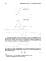
FIGURE 18.1 Typical progression of a force-directed placement method for the circuit IBM04 from the

ICCAD04 mixed-size placement benchmark suite: (a)initial placement, (b) after roughly1/3 through placement,
(c) after roughly 2/3 through placement, and (d) before legalization and detailed improvement. The fairly
nonoverlapping placement before legalization is obtained without the use of partitioning.
Force-directed methods differ from other placement methods, including simulated annealing,
minimum-cut, and analytic methods. Simulated annealing typically begins with an initial feasible
(or nearly feasible) placement and applies iterative improvement. Conversely, force-directed methods
typically begin with no initial placement and construct the placement as they progress. Minimum-
cut and analytic methods are also constructive, but rely on partitioning of the placement area to
remove cell overlap. Force-directed methods, however, do not use partitioning, but rather eliminate
cell overlap through the introduction of repulsive forces.
The earliest implementations of force-directed methods were examined in the 1960s [2], and
many adaptations of these methods remain in use today. Although many variations exist, it is a
proper understanding of the similarities and differences between the methods that can lead to either
a successful or unsuccessful implementation.
In this chapter, we examine force-directed methods by considering how some of these work. We
do not make comparisons between the methods, but rather attempt to illustrate the issues, similarities,
and differences between the various implementations described in the literature. We also exam ine
other continuous placement methods (i.e., methods that do not rely on partitioning to remove cell
overlap) that, although not seemingly force-directed, still share characteristics with force-directed
methods. This chapter is organized as follows. In Section 18.2, we describe the traditional force-
directed method that employs quadratic optimization to minimize wirelength and additional constant
forces to remove cell overlap. We d escribe methods that use techniques other than constant forces
Alpert/Handbook of Algorithms for Physical Design Automation AU7242_C018 Finals Page 349 23-9-2008 #4
Force-Directed and Other Continuous Placement Methods 349
to eliminate cell overlap in Section 18.3. This includes fixed-point and frequency-based methods.
Quadratic optimization is not the best choice for high-quality placemen ts. Many force-d irected
methods are used in combinationwith other optimizationstrategies—wetouch upon theseinterleaved
optimizations in Section 18.4. In Section 18.5, we describe other continuous placement techniques
and describe their relationships with force-directed methods. Section18.6 describes several issues
facing force-directed methods, and Section 18.7 offers concluding remarks.

18.2 BASIC ELEMENTS OF FORCE-DIRECTED PLACEMENT
Placement typically begins with a circuit netlist modeled as a hypergraph G
h
(V
h
, E
h
) with vertices
V
h
={v
1
, v
2
, , v
n
, v
n+1
, , v
n+p
} representing circuit cells and hyperedges E
h
={e
1
, e
2
, , e
m
}
representing circuit nets. The set {v

1
, v
2
, , v
n
} represents movable cells and the set {v
n+1
, , v
n+p
}
represents preplaced cells and I/O pads. Each vertex v
i
has dimensions w
i
and h
i
that represent the
width and height of its corresponding circuit cell, respectively. Let (x
i
, y
i
) denote the coordinates
of th e center of vertex v
i
. Placement information is then captured in the x-andy-directions by two
placement vectors x = (x
1
, x
2
, , x

n
) and y = (y
1
, y
2
, , y
n
).
Placement seeks to optimize objectives, including the minimization of total interconnect length,
routing congestion, power consumption, and timing requirements, subject to the constraint that cells
cannot overlap. Of course, the simultaneous optimization of these different objectives is difficult.
Wirelength is one of the most commonly employed measures of quality—the minimization of wire-
length tends to be simpler a nd also aids in the minimization of other objectives. The most commonly
used measurement of wirelength in modern placement is the half-perimeter wirelength (HPWL),
which, for any given net e ∈ E
H
, is the minimum rectangle that encloses all cells on net e and can be
written as
HPWL(e) = max
i,j∈e,i <j
|x
i
− x
j
|+max
i,j∈e,i <j
|y
i
− y
j

| (18.1)
The totalwirelength of thecircuit isgiven by

e∈E
H
HPWL(e). AlthoughHPWL is a convex function,
it is neither strictly convex nor differentiable because of the absolute d istances |x
i
−x
j
|and |y
i
−y
j
|—
its direct and efficient minimization is difficult. Placement f ocuses on minimizing an approximation
of HPWL subject to the constraint that no cells may overlap. In practice, HPWL is a reasonably close
approximation to the final, routed wirelength [3].
18.2.1 QUADRATIC OPTIMIZATION PRELIMINARIES
Kraftwerk [4], perhaps the best-known force-directed placer, introduced a quadratic approxima-
tion [5] to HPWL and many other placers have since followed its lead. In quadratic placement, the
circuit hypergraphis transformed into a weighted graph. Such a transformation necessitates that each
hyperedge be modeled as a set of two-pin nets using a suitable net model. Typical net models include
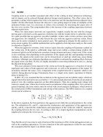
clique or star models, as shown in Figure 18.2 for a five-pin net. In the clique model, each k-pin net
is replaced by k(k − 1)/2 two-pin nets. In the star model, a star node is added for each net to which
all pins of the nets are connected. If the weight of a k-pin hyperedge is W, it is common to weight
the set of two-pin nets using a weight such as W /(k − 1) [6].
The selection of the net model is an implementation decision. It is typical to use a clique model
for small nets with few pins, but to switch to the star model for nets with a large number of pins.
The clique model results in a denser quadratic optimization problem, whereas the star model tends

to improve the sparsity of the problem, but requires additional dummy cells to represent the star
nodes. At first glance, it might appear that the choice of net model can influence the solution to the
placement problem and this observation is generally true. However, it has been demonstrated [7–9]
that weights for the clique and star models can be selected such that the placement solutions are
Alpert/Handbook of Algorithms for Physical Design Automation AU7242_C018 Finals Page 350 23-9-2008 #5
350 Handbook of Algorithms for Physical Design Automation
(a) (b)
Star node
FIGURE 18.2 Models for a five-pin net in which the net is modeled as a (a) clique or as a (b) star. In both
cases, the edges in the net model can be weighted. (From Viswanathan, N. and Chu, C.C N., IEEE Trans. CAD
24, 5, 722, 2005. Copyright IEEE 2005. With permission.)
identical regardless of the model used. Without any loss of generality, we will assume a clique model
for all nets in the remainder of our discussion.
∗
A quadratic placement can be obtained by minimizing the unconstrained objective function
given by
(x, y) =

i,j
w
i,j
[(x
i
− x
j
)
2
+ (y
i
− y

j
)
2
] (18.2)
where w
ij
represents the weight on the two-pin edge connecting cells i and j in the circuit’s weighted
graph representation. This objective function is separable into (x, y) = (x) + (y) and can be
written in matrix notation (x-direction only) given by
(x) =
1
2
x
T
Q
x
x +c
T
x
x +const (18.3)
The n
x
× n
x
Hessian matrix Q
x
encapsulates the connections between pairs o f m ovable cells and is
symmetric positive definite.
†
Vector c

x
encapsulates connections between movable cells and fixed
cells. Finally, the constant is a result of connections to and between fixed cells. Equation 18.3 is
minimized by solving the positive definite system of linear equations given by
Q
x
x +c
x
= 0 (18.4)
and is typically solved using any number of iterative solvers including CG, SYMMLQ, GMRES,
BICGSTAB, and so forth [10]. Matrix preconditioning is also used to improve the overall efficiency
of the iterative solver, including ILU, drop tolerance, and random walk preconditioners [10,11].
Quadratic optimizationis oftenreferredtoas force-directedplacement.Such ananalogyfollowsif
the weighted two-pin nets in the circuit’s graph approximation are viewed as springs. We can consider
the netlist as a system of objects connected by springs with different spring constants (weights).
Minimizing the quadratic objective is equivalent to putting the system into a force-equilibrium state
in which the resultant force on each movable cell owing to all of the connected spring forces is
zero. This result stems from Equation18.4, in which the ith row of the system of linear equations
represents the resultant force o n cell i being set to zero.
∗
We note that models based on Steiner trees [12], multipin net decomposition [13], and bounding box [14] have also been
suggested in the literature; we refer interes ted readers to these sources for more information.
†
Positive definiteness requires the presence of fixed cells [5,15]. Further, fix ed cells are required for a unique s olution to the
optimization problem.
Alpert/Handbook of Algorithms for Physical Design Automation AU7242_C018 Finals Page 351 23-9-2008 #6
Force-Directed and Other Continuous Placement Methods 351
Unfortunately, solving Equation 18.4 results in a cell placement with significant cell overlap.
For example, Figure 18.1a shows the placement for circuit IBM04 from the ICCAD04 mixed-size
placement benchmark suite [1] after the solution of an unconstrainedquadratic program—significant

cell overlap clearly exists.
18.2.2 FORCE-BASED SPREADING
Both Kraftwerk and FDP [16] apply additional constant forces to reduce cell overlap. The force
Equation18.4 is extended with an additional constant force vector f
x
yielding
Q
x
x +c
x
+ f
x
= 0 (18.5)
The vector f
x
is used to perturb the placement such that cell overlap is reduced. It is easy to show
that the additional forces do not restrict the solution space and that any given placement can satisfy
Equation18.5 by proper selection of f
x
[4].
Cell overlap is not removed just by solving a single perturbation of Equation18.4 by Equa-
tion 18.5. Instead, the cell overlap is removed over numerous iterations with the additional constant
forces being updated at each iteration to reflect the changing distribution of cells throughout the
placement area. Hence, the additional constant forces are accumulated over iterations and the force
equation at any given iteration i can be written as
Q
x
x
i
+ c

x
+
i−1

k=1
f
k
x
+ f
i
x
= 0 (18.6)
The additionalconstant force isdividedinto twoparts, namely thoseforcesaccumulated overprevious
placement iterations 1 through i−1 and a current constant force computedat iteration i. Equivalently,
the additional constant force computed at any given iteration is broken into two specific components,
namely (1) a stabilizing force that holds the current placement in equilibrium (represented by the
accumulation of forces from previous iterations) and (2) a perturbing force computed for a given
placement to further reduce cell overlap.
In addition to the requirement that the additiona l forces be used to distribute cells evenly
throughout theplacement area, Ref.[4]specifiesadditional requirementsthat theforces mustsatisfy:
1. Force on a cell depends only on its position.
2. Overutilized regions of the placement area are sources of forces.
3. Under-utilized regions of the placement area are sinks of forces.
4. Forces should not form circles.
5. Forces should be zero at infinity.
Given these requirements, the force f (x, y) acting on a cell at position (x, y) within the placement
region is computed using Poisson’s equation given by
∂
2
φ(x, y)

∂x
2
+
∂
2
φ(x, y)
∂y
2
= κd(x, y) (18.7)
where
d(x, y) is a measure of density at position (x, y)
κ is a constant of proportionality
φ(x, y) is a scalar function such that ∇φ(x, y) = f (x, y)