Handbook of algorithms for physical design automation part 51 pptx

Alpert/Handbook of Algorithms for Physical Design Automation AU7242_C023 Finals Page 482 23-9-2008 #15
482 Handbook of Algorithms for Physical Design Automation
1
1
1
1
1
1
1
2
2
2
2
2
2
C
A
C
A
C
BBB
A
2
1
1
1
2
22
2
2
3

3
33
3
3
3
321
4
4
4
4
4
4
4
4
5
5
5
5
5
5
5
5
5
6
6
6
6
6
6
6

6
6
6
7
7
7
7
7
7
7
7
7
7
7
8
8
8
8
8
8
8
8
8
8
8
8
9
9
9
99

9
9
9
9
9
9
9
1111
11
1
1
111
1
1
1
1
1
2
2
2
2
2
2
2
2
2
2
2
2
2

22
3
3
33
3
3
3
3
3
3
3
3
3
3
3
3
3
3
3
4
4
4
4
4
4
4
4
4
44
4

4
4
4
4
4
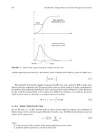
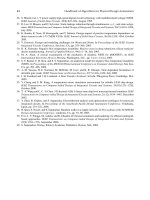
(a) (b) (c)
FIGURE 23.17 Maze routing is applied repeatedly to find the routing solution of a net with three terminals.
(a) Wave expansion starts from terminal A, and it reaches terminal B; (b) the route between A and B is
implemented, and the new wavefront is expanded from the partial route; and (c) the final routing solution
obtained.
the wave expansion. In other words, the next wavefront is expanded starting from the partial route
implemented. This process continues until all the terminals of the net are routed. Figure 23.17
illustrates this process with an example. Here, wave expansion starts from terminal A, and it reaches
terminal B (Figure 23.17a). Then, the route between A and B is implemented by backtracking. The
next wavefront is started to be expanded from this partial route (Figure 23.17b). Finally, the new
wavefront reaches C, and the final solution is obtained. Note here that this approach can easily lead
to suboptimal solutions because of its greedy nature. For example, if the lower L route was selected
in Figure 23.17b as the route between A and B, then the wirelength of the final routing solution would
be significantly larger. To avoid this problem, a biasing technique is proposed in Ref. [41] to direct
the maze search toward regions where overlap with future connections of the net is more likely.
23.6 ROUTING MULTIPLE NETS
In this section, we focus on the problem of routing multiple nets together. The main difficulty here
is that routing solution for one net potentially impacts the routing of o ther nets, because common
routing resources are being used by multiple nets. We can divide the routing methodologies that deal
with multiple nets into two broad categories: sequential and concurrent routing methodologies. In
the following subsections, we give a brief overview of these techniques.
23.6.1 SEQUENTIAL ROUTING
The most straightf orwardway of routing multiple nets is to route them sequentially in a specific order.
Once a net is routed, the congestion values of the global routing resources being used are updated. As
a result, some of the nets to be routed in the later iterations may be forced to use overcongested routing

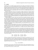
resources. So, this approach is very sensitive to the order of nets that are being routed. Figure 23.18
illustrates an example where net ordering has an impact on the final solution. In Figure 23.18a, net
C is routed after nets A and B, and its path is blocked by the other routing segments. This leads to an
overcongested solution. In Figure 23.18b, net A is routed after nets C and B, and all its shortest paths
are blocked by the other routing segments. This leads to a solution with suboptimal wirelength for
net A. In Figure 23.18c, the best net ordering is illustrated, which leads to a congestion-free routing
solution with optimal routing for each net.
Several practical considerations are taken into account while making the net ordering decision.
The nets that have highe r criticalities are typically routed first so that they have high e r priorities
while using contentious routing resources. The criticality of a net is determined by th e importance of
the net and the timing requirements imposed on it. For example, if a net is on the critical path of the
circuit, it can be prioritized so that it uses the fastest routing resources before they are acquired by
Alpert/Handbook of Algorithms for Physical Design Automation AU7242_C023 Finals Page 483 23-9-2008 #16
Global Routing Formulation and Maze Routing 483
A
C
C
B
B
A
A
C
C
B
B
A
A
C
C
B

B
A
(a) (b) (c)
FIGURE 23.18 Net ordering problem is illustrated for three nets. The capacity of each tile is assumed to
be one vertical and one horizontal track. Routing nets in the order (a) A–B–C leads to a solution with two
overcongested tiles (shown as shaded rectangles), (b) C–B–A leads to a solution where A is detoured to avoid
congestion, and (c) C–A–B leads to the congestion-free solution with optimal routing for each net.
other nets. Another practical consideration is routing nets with less routing alternatives before other
nets. Typically, routing choices are limited for the nets of which terminals are close to each other.
Similarly, if all the terminals of a net align with each other on one row or column of the routing g rid
(e.g., net C in Figure 23.18), then routing choices will be limited for such a net. So, it is a commonly
used heuristic to determine net ordering based on increasing Manhattan distances of the terminals.
The main disadvantage of sequential routing methodologies is that the n ets that are routed earlier
affect the routing of the latter nets. To alleviate this problem, rip-up and reroute techniques [42,43]
are used so that the nets that are routed in the earlier iterations can be rerouted based on the routing
requirements of the latter nets. Typically, nets are first routed allowing congestion, and then the
nets in the overcongested regions are ripped up and rerouted in the later iterations. For example in
Figure 23.18a, nets are routed in the order A–B–C. Here, if net A is ripped up and rerouted, it will
prefer the uncongested region, and the solution in Figure 23.18b will be obtained.
A problem with the rip-up- and rero ute-based algorithms is solution oscillations. It is possible
that the congestion will oscillate between two regions during the routing iterations as nets are being
ripped up and rerouted. To avoid this problem, some algorithms incorporate the congestion history
into the routing objective function. Pathfinder is a negotiated-congestion-based algorithm, which
was proposed for FPGA routing [44–46], and extended to different aplication areas such as PCB
routing [47]. Recently, global routing algorithms have been proposed that utilize congestion histories
[23,25,48], and outperform other algorithms on recently released public benchmarks [49]. The main
idea of congestion negotiation can be summarized as follows. First, every net is routed individually,
regardless of any overuse (i.e., congestion) of routing grid edges. Then the n ets are ripped up and
rerouted one by one iteratively. In each iteration, the congestion cost of each edge is updated based
on the current and past overuse of it. By increasing the congestion cost of an overused edge gradually,

the nets with alternative routes are forced not to use this edge. Eventually, only the net that needs
to use this edge most ends up using it. For example, Archer [23] uses the following cost function to
compute the congestion history of edge e:
cost(e) = (1 +α.h
k
e
) ×overflow (e) (23.1)
Here, h
k
e
represents the history cost for edge e in iteration k, and it reflects for how long edge e has
been congested. It is computed as follows:
h
k
e
=

h
k−1
e
if edge e is congestion free in iteration k
h
k−1
e
+ k if edge e has nonzero overflow in itera tion k
(23.2)
Alpert/Handbook of Algorithms for Physical Design Automation AU7242_C023 Finals Page 484 23-9-2008 #17
484 Handbook of Algorithms for Physical Design Automation
Based on this formulation, if edge e is congested repeatedly for several iterations, its cost will
increase significantly to discourage its usage. Aging effect is also captured by this formulation. The

edges that are congested only in the earlier iterations will have less costs than the ones that are
congested in the later iterations.
In Chapter 31, a more thorough survey of rip-up and reroute algorithms is provided.
23.6.2 CONCURRENT ROUTING
The sequential routing algorithms are commonly used mainly because of their simplicity and low-
runtime requirements. However, they are heuristics-based, and they typically do not have any
theoretical guarantee about solution quality. As discussed in the previous section, the order in which
nets are routed typically affects the routing results of sequential algorithms significantly. For the pur-
pose of avoiding this problem, another class of algorithms try to find the routing solutions of all nets
concurrently. In this subsection , a brief overview of routing formulations based on multicommodity
flow and integer linear programming will be given.
Global routing problem can be formulated as a multicommodity flow problem as follows. Let
G = (V, E) b e the global routing graph with vertices V and edges E. A flow network can be modeled
based on this graph G. Each edge e ∈ E in this network will have flow capacity cap(e) (which can
be set based on the techniques presented in Section 23.3), and cost cost(e) (which can be set based
on the cost metrics discussed in Section 23.4). A commodity must be transported over this network
corresponding to each net between the vertices corresponding to its terminals. The multicommodity
flow problem is defined as finding a flow f or each commodity between specified vertices while
satisfying all flow capacity constraints of the edges in the network. There are two variations of
this problem depending on whether fractional flow values on edges are allowed or not. While the
fractional multicommodity flow problem is polynomial-timesolvable, integer multicommodity flow
problem is NP-complete.
Shragowitz et al. [50] present one of the earlier global routing algorithms that uses multicom-
modity flow formulation for two-terminal nets. Raghavan et al. [51] present an improved network
flow formulation that can also handle three-terminal nets. A more recent algorithm proposed by
Albrecht [18] operates on a set of given Steiner trees T
i
for each net i with the objective of choosing
exactly one T ∈ T
i

such that the maximum relative congestion in the circuit is minimized. The
readers can refer to Chapter 32 for a more detailed survey of concurrent routing algorithms.
23.7 CONCLUSIONS
In this chapter, we have discussed the basics of global routing. As discussed before, global routing
is an important step in the physical design process, and it impacts the final interconnect qualities
considerably. As the circ uit densities have been significantly increasing in the past several years,
the routing problem for integrated circuits is becoming a more and more challenging problem.
A recent global routing competition in ISPD 2007 [49] attracted renewed interest in global rout-
ing, and the results of the recently proposed algorithms [23,25,48] demonstrated that there is still
significant room for routing quality improvements.
The next two chapters provide detailed discussions on net-topology optimization techniques for
multiterminal nets. Although these chapters focus on single-net optimization, they can be utilized
within a global routing framework to determine net topologies, as discussed in Section 23.5.5.
REFERENCES
1. G. W. Clow. A global routing algorithm for general cells. In 21st Design Automation Conference, IEEE
Press, Piscataway, NJ, pp. 45–51, 1984.
2. J. Cong and P. M adden. Performance driven global routing for standard cell design. In International
Symposium on Physical Design, ACM, NY, pp. 73–80, 1997.
Alpert/Handbook of Algorithms for Physical Design Automation AU7242_C023 Finals Page 485 23-9-2008 #18
Global Routing Formulation and Maze Routing 485
3. J. T. Mowchenko and C. S. R. Ma. A new global routing algorithm for standard cell ICs. In International
Symposium on Circuits and Systems, pp. 27–30, 1987.
4. C. Sechen and A. Sangiovanni-Vincentelli. Timberwolf 3.2: A new standard cell placement and global
routing package. In 23rd Design Automation Confer ence, IEEE Computer Society Press, Lo s Alamitos,
CA, pp. 432–439, 1986.
5. J. Cong and B. Preas. A new algorithm for standard cell global routing. Integration: The VLSI Journal,
14(1): 49–65, 1992. (ICCAD 1988.)
6. W. Sw artz and C. Sechen. A new generalized row-based global router. International Conference on
Computer Aided Design, IEEE Computer Society Press, Los Alamitos, CA, pp. 491–498, 1993.
7. M. Burstein and R. Pelavin. Hierarchical channel router. In Proceedings of 20th Design Automation

Conference, ACM, NY, pp. 591–597, 1983.
8. S. C. Fang, W. S. Feng, and S. L. Lee. A new efficient approach to multilayer channel routing problem. In
Pr oceedings of the 29th Design Automation Conference, IEEE Computer Society Press, Los Alamitos, CA,
pp. 579–584, 1992.
9. A. Hashimoto and J. Stevens. Wire routing by optimizing channel assignment within large apertures. In
Pr oceedings of the 8th Desi gn Automation Workshop, A CM, NY, pp. 214–224, 1971.
10. M. M. Ozdal and M. D. F. Wong. Two layer bus routing for high-speed printed circuit boards. ACM
Transactions on Design Automation of Electronic Systems, 11(1): 213–227, 2006. (ICCAD 2004.)
11. R. L. Rivest and C. M. Fiduccia. A greedy channel router. In Proceedings of 19th Design Automation
Conference, IEEE Press, Piscataway, NJ, pp. 418–424, 1982.
12. T. Yoshimura. Efficient algorithms for channel routing. IEEE Transactions on Computer-Aided Design,
CAD-1(1): 25–35, 1982.
13. C. Hsu. General river routing algorithm. In Proceedings of 20th Design Automation Conference, IEEE
Press, Piscataway, NJ, pp. 578–582, 1983.
14. M. M. Ozdal and M. D. F. Wong. Algorithmic study of single-layer bus routing for high-speed boards.
IEEE Transactions on Computer-Aided Design of Integrated Cir cuits and Systems, 25(3): 490–503, 2006.
(ICCAD 2004.)
15. R. Y. Pinter. On routing two -point nets across a channel. In Pr oceedings of 19th Design Automation
Conference, IEEE Press, Piscataway, NJ, pp. 894–902, 1982.
16. R. Y. Pinter. River r outing: Methodology and analysis. I n Proceedings of 3rd Caltech Conference on VLSI,
Computer Science Press, pp. 141–163, 1983.
17. H. Zhou and M. D. F. Wong. Optimal river routing with crosstalk constraints. ACM Transactions on Design
Automation of Electronic Systems, 3( 3): 496–514, 1998.
18. C. Albrecht. Provably good global routing by a new approximation algorithm for multicommodity flow.
In I n ternational Symposium on Physical Design, ACM, NY, pp. 19–25, 2000.
19. M. Cho and D. Z. Pan. Boxrouter: A new global router based on box expansion and progressive ilp.
In Proceedings of Design Automation C onference, ACM, N Y, pp. 373–378, 2006.
20. R. T. H adsell and P. H. Madden. Improved global routing through congestion e stimation. In Proceedings
of Design Aut omation Conference , ACM, NY, pp. 28–31, 2003.
21. R. Kastner, E. Bozorgzadeh, and M. Sarrafzadeh. Predictable routing. In Proceedings of International

Conference on Computer Aided Design, IEEE Press, Piscataway, NJ, pp. 110–114, 2000.
22. R.Kastner, E.Bozorgzadeh,andM. Sarrafzadeh. Patternrouting: Use andtheory forincreasing predictability
and avoiding coupling. IEEE Transactions on C omputer Aided Design of Integr ated Circuits and Systems,
21(7): 777–791, 2002.
23. M. M. O zdal a nd M. D. F. Wong. Archer: A history-driven global routing algorithm. In Proceedings of
International Conference on Computer Aided Design, IEEE P ress, Piscataway, NJ, pp. 488–495, 2007.
24. M. Pan and C. Chu. Fastroute: A step to integrate global routing into placement. In Proceedings of
International Conference on Computer Aided Design, IEEE P ress, Piscataway, NJ, pp. 464–471, 2006.
25. J.A. Royand I. L. Mark ov. High-performance routingat the nanometer scale. In Pr oceedings of International
Conference on Computer Aided Design, IEEE Press, Piscataway, NJ, pp. 496–502, 2007.
26. J. Cong, J. Fang, and K. -Y. Khoo. DUNE: A multi-layer gridless routing system. IEEE Transactions on
Computer-Aided Design of In tegrated Circuits and Systems,
20(
5): 633–647, 2001. (ISPD 2000).
27. J. Cong, J. Fang, M. Xie, and Y. Zhang. MARS: A multilevel full-chip gridless routing system. IEEE
Transactions on Computer-Aided Design of Integrated Circuits and Systems, 24(3): 382–394, 2005. (ICCAD
2002.)
Alpert/Handbook of Algorithms for Physical Design Automation AU7242_C023 Finals Page 486 23-9-2008 #19
486 Handbook of Algorithms for Physical Design Automation
28. J. Cong and P. H. Madden. Performance driven multi-layer general area routing for PCB/MCM designs. In
Pr oceedings of Design Automation C onference, ACM, N Y, pp. 356–361, 1998.
29. R. Linsker. An iterative-improvement penalty-function-drivenwire routing system. IBM Journal of Research
and Development, 28(5): 613–624, 1984.
30. H. Zhou and M. D. F. Wong. Global routing with crosstalk constraints. In Proceedings of Design Automation
Conference, ACM, NY, pp. 374–377, 1998.
31. C. Y. Lee. An algorithm for path connection and its applications. IRE Tr ansactions on Electronic Computers,
EC-10: 346–365, 1961.
32. E. F. Moore. The shortest path through a maze. In Proceedings of the International Symposium on the
Theory of Switching, pp. 285–292. Harvard University Press, Cambridge, 1959.
33. S. Akers. Routing, Vol. 1. Prentice-Hall, Englewood Cliffs, NJ, 1972.

34. S. Akers. A modification of lee’s path connection algorithm. IEEE Transactions on Electronic Computers,
EC-16(2): 97–98, 1967.
35. F. O. Hadlock. A shortest path algorithm for grid graphs. Networks, 7(4): 323–334, 1977.
36. P. E. Hart, N. J. Nilsson, and B. Raphael. A formal basis for the heuristic determination of minimum cost
paths in graphs. IEEE Transactions on Systems Science and Cybernetics, SSC-4(2): 100–107, 1968.
37. J. Soukup. Fast maze router. In Proceedings of the 15th Design Automation Conference, IEEE Press,
Piscataway, NJ, pp. 100–102, 1978.
38. E. W. Dijkstra. A note on two problems in connection with gr aphs. Numerische Mathematik, 1: 269–
271, 1959.
39. K. Mikami and K. Tabuchi. A computer program for optimal routing o f printed ci rcuit connectors. In IFIPS
Pr oceedings, H47: 1475–1478, 1968.
40. D. W. Hightower. A solution to line-routing problems on the continuous plane. In Pr oceedings of the 6th
Annual Conference on Design Automation, ACM, NY, pp. 1–24, 1969.
41. R. F. Hentschke, J. Narasimham, M. O. Johann, and R. L. Reis. Maze routing steiner trees with effective
critical sink optimization. In Pr oceedings of International Symposium on Physical Design,ACM,NY,
pp. 135–142, 2007.
42. H. Bo llinger. A mature DA system for PC layout. In Proceedings of 1st International Printed Circuit
Conference, IEEE Computer Society Press, Los Alamitos, CA, pp. 85–99, 1979.
43. W. A.Dees and P. G. Karger. Automated rip-up a ndreroute techniques. In Proceedings of Design Automation
Conference, IEEE Press, Piscataway, NJ, pp. 432–439, 1982.
44. V. Betz and J. Rose. D irectional bias and non-uniformity in FPGA global routing architectures.
In International Confer ence on Computer Aided Design, IEEE Computer Society, Washington, DC,
pp. 652–659, 1996.
45. V. Betz andJ. Rose. VPR: Anewpacking, placement androuting tool for FPGA research. In7th International
Workshop on Field-Progr ammable Logic, pp. 213–222, 1997.
46. C. Ebeling, L. McMurchie, S. A. Hauck, and S . Burns. Placement and routing tools for the triptych FPGA.
IEEE Transactions on VLSI Systems, IEEE Press, Piscataway, NJ, pp. 473–482, 1995.
47. M. M. Ozdal and M. D. F. Wong. A length-matching r outing algorithm for high-performance printed circuit
boards. IEEE Tr ansactions on Computer-Aided Design of Integrated Circuits and Systems (TCAD), 25:
2784–2794, 2006. (ICCAD 2003).

48. M. Cho, K. Lu, and D. Z. Pan. Boxrouter 2.0: Architecture and implementation of a hybrid and robust
global router. In Proceedings of International Conference on Computer Aided Design, Press, Piscataway,
NJ, pp. 503–508, 2007.
49. G. -J. Nam. ISPD 2007 Global Routing Contest, 2007. Available at: />contest.html
50. E. Shragowitz and S. Keel. A global router based on a multicommodity flow model. Integration: The VLSI
Journal, 5(1): 3–16, 1987.
51. P. Raghavan and C. D. Thompson. Multiterminal global routing: A deterministic approximation scheme.
Algorithmica, 6: 73–82, 1991.
Alpert/Handbook of Algorithms for Physical Design Automation AU7242_C024 Finals Page 487 9-10-2008 #2
24
Minimum Steiner Tree
Construction*
Gabriel Robins and Alexander Zelikovsky
CONTENTS
24.1 Introduction 487
24.2 Historical Perspectives 489
24.3 Iterated 1-Steiner Approach 490
24.3.1 Batched 1-Steiner Variant 492
24.3.2 Empirical Performance of Iterated 1-Steiner 493
24.3.3 Generalization of I1S to Steiner Arborescences 494
24.4 Steiner Trees in Graphs 494
24.4.1 Graph Generalization of Iterated 1-Steiner 494
24.4.2 Loss-Contracting Approach 495
24.5 Group Steiner Trees 496
24.5.1 Applications of GroupSteiner Trees 497
24.5.2 Depth-Bounded Group Steiner Tree Approach 498
24.5.3 Time Complexity of the DBS Group Steiner Algorithm 499
24.5.4 Degenerate Group Steiner Instances 500
24.5.5 Bounded-Radius Group Steiner Trees 501
24.5.6 Empirical Performance of the Group Steiner Heuristic 502

24.6 Other Steiner Tree Methods 502
24.7 Improving the Theoretical Bounds 502
24.8 Steiner Tree Heuristics in Practice 503
24.9 Future Directions for the Steiner Problem 503
References 504
24.1 INTRODUCTION
In optimizing the area of very large scale integrated (VLSI) layouts, circuit interconnections should
generally be realized with minimum total interconnect. This chapter addresses several variations
of the corresponding fundamental Steiner minimal tree (SMT) problem, where a given set of pins
is to be connected using minimum total wirelength. Steiner trees are important in global routing
and wirelength estimation [1], as well as in various nonVLSI applications such as phylogenetic
tree reconstruction in biology [2], network routing [3], and civil engineering, among many other
areas [4–9].
In modern deep-submicron VLSI layout other criteria often dominate the routing objectives,
such as pathlengths, skew, density, inductance, manufacturability, electromigration,reliability, noise,
∗
This work was supported b y a Packard Foundation Fellowship, by National Science Foundation Young Investigator Award
MIP-9457412, by a GSU Research Initiation Grant, by NSF grants CCR-9988331, CCF-0429737, CCF-0429735, and
CNS-0716635, and by U.S. Civ ilian Research and Development Foundation grant MOM2-3049-CS-03.
487
Alpert/Handbook of Algorithms for Physical Design Automation AU7242_C024 Finals Page 488 9-10-2008 #3
488 Handbook of Algorithms for Physical Design Automation
power, non-Hanan topologies, signal integrity, three-dimensionality, alternate models, and vari-
ous combinations and trade-offs of these Refs. [10–22]. However, large noncritical nets are still
common in modern designs, and this chapter focuses on the corresponding classical objective of
wirelength/area minimization (which also minimizes the total capacitance). This exposition is not
an exhaustive survey on the Steiner problem, about which hundreds of papers and several entire
books were written [2,4–9]. Rather, it focuses o n a few selected results and approaches to Steiner
tree construction. A broader overview of the field of computer-aided design of VLSI is given by
several textbooks on this subject [23–27].

Given a set P of n pins (i.e., terminals of a signal net), we seek to interconnect these points using a
minimual total amount of wire. This objective arises in VLSI minim um-area global routing, because
VLSI minimum-spacing design rules induce an essentially linear relationship between wirelength
and wiring area. When all wires are point-to-point, with no intermediate junctions other than points
of P, the optimum solution is a minimum spanning tree (MST) over P, denoted as MST(P). However,
we can usually introduce intermediate junctions, called Steiner points, in connecting the points of P.
The SMT problem can be formulated as follows.
Steiner minimal tree problem: Given a set P of n points, determine a set S of Steiner points such that
the MST cost over P ∪S is minimized.
An optimal solution to this problem is referred to as a SMT (or simply Steiner tree) over P,
denoted SMT(P). An edge in a tree T has cost equal to the distance between its endpoints, and the
cost of T itself is the sum of its edge costs, denoted cost(T). The wiring cost between a pair of pins
(x
1
, y
1
) and (x
2
, y
2
) in a VLSI layout is typically modeled by the Manhattan or rectilinear distance:
∗
dist

(
x
1
, y
1
)

,
(
x
2
, y
2
)

= (x) +(y) =
|
x
1
− x
2
|
+
|
y
1
− y
2
|
We will focus on the rectilinear SMT problem, where every edge is embedded in the plane
using a path of one or more alternating horizontal and vertical segments between its endpoints.
Figure 24.1 depicts an MST and an SMT for the same pointset in the Manhattan plane. The bounding
box of a pointset P denotes the smallest rectangle,
†
which contains all points of P and whose
sides are oriented parallel to the coordinate axes. If an edge between two points is embedded with
minimum possible wirelength, its routing segments will remain within the bounding box induced by

its endpoints.
(a) (b)
FIGURE 24.1 (a) MST and (b) SMT in the rectilinear plane. Hollow dots represent the original pointset P,
and solid dots represent Steiner points.
∗
More recently, non-Manhattan interconnect architectures such as preferred direction routing and λ-geometries, have been
gaining popularity [4,28–36]. Howe ver, most of the m e thods described i n this chapter can be generalized to these o ther
geometries and metrics, as well as to higher dimensions.
†
Bounding boxes in non-Manhattan metrics/geometries havecorresponding nonrectangular shapes, inducedby theunderlying
metric/geometry [4].
Alpert/Handbook of Algorithms for Physical Design Automation AU7242_C024 Finals Page 489 9-10-2008 #4
Minimum Steiner Tree Construction 489
24.2 HISTORICAL PERSPECTIVES
The Steiner problem is named after the Swiss mathematician Jacob Steiner (1796–1863),who solved
and popularized the problem of joining three villages by a system of roads having minimum total
length [37](he also addressedthegeneral case of this problem, andmade many fundamentalcontribu-
tions to projectivegeometry).However,while Jacob Steiner’s work on this problem was independent
of its predecessors, about two centuries earlier Pierre de Fermat (1601–1665) proposed this problem
to Evangelista Torricelli (1608–1647), who solved it and passed it along to his student Vincenzo
Viviani (1622–1703), who in turn published his own solution as well as Torricelli’s in 1659 [38].
An even earlier (and presumably independent) published discussion of this problem is found in a
1647 book by the Italian mathematician Bonaventura Francesco Cavalieri (1598–1647) [39]. Luck-
ily, today we refer to this problem simply as the Steiner problem, instead of the more accurate but
considerably less wieldy title the Fermat–Torricelli–Viviani–Cavalieri–Steiner problem.
More recent research progress on the SMT problem has been historically driven by several
main results.
1. In 1966, Hanan [40] showed that for a pointset P there exists an SMT whose Steiner points S
are all chosen from the Hanan grid, namely the intersectionsofall the horizontaland vertical
lines passing through every point of P (Figure 24.2). Snyder [41] generalized Hanan’s

theorem to all higher dimensional Manhattan geometries; on the other hand, extensions of
Hanan’s theorem to λ-geometries are less straightforward [42].
2. In 1977, Garey and Johnson showed that despite restricting the Steiner points to lie on the
Hanan grid, the rectilinear SMT problem is NP-complete [43 ]. Only a very few special
cases have been solved optimally (e.g., a linear-time solution exists when all points of P lie
on the boundary of a rectangle [44]). Many heuristics have been proposed for the general
problem, as surveyed in Refs. [2,5–8].
3. In 1976, Hwang [45] showed that the MST over P is a good approximation to the SMT,
having performance ratio
∗
cost[MST(P)]
cost[SMT(P)]
≤
3
2
for any pointset P in the rectilinear plane. In
attacking intractable problems, a standard goal is to achieve a provably good heuristic
having a constant-factor performance ratio (i.e., asymptotic worst-case error bounded with
respect to the optimal solution) . In light of the intractability of the rectilinear SMT problem,
Hwang’s result implies that any Steiner approximation approach that improves upon an
initial MST solution will have performance ratio at most
3
2
. Thus, many SMT heuristics in
the literature are MST-improvement strategies, i.e.,they resembleclassicMST con structions
(e.g., Refs. [46,47]).
For over 15 years after the publication of Ref. [45], the fundamental open p roblem was
to find a heuristic with (worst-case) performance ratio strictly less than
3
2

. A complementary
FIGURE 24.2 Hanan’s theorem: There exists an SMT with Steiner points chosen from the Hanan grid, i.e.,
intersection points of all hor izontal and vertical lines drawn through the points.
∗
The p erformance ratio of a heuristic is an upper bound on the heuristic solution cost d ivided by the optimal s olution cost,
over all possible problem inst ances

i.e., the worst-case of
cost(APPROX)
cost(OPT)

.
Alpert/Handbook of Algorithms for Physical Design Automation AU7242_C024 Finals Page 490 9-10-2008 #5
490 Handbook of Algorithms for Physical Design Automation
research goal has been to find new practical heuristics with improved average-case solu-
tion quality. In practice, most SMT heuristics, including MST-based strategies, exhibited
very similar average performance. On uniformly distributed random instances (the typical
benchmark), heuristic Steiner tree costs averaged between 7 and 9 percent improvement
over the corresponding MST costs [2].
4. In 1990, Kahng and Robins have shown [19,48–50] that any Steiner tree heuristic in a
general class of greedy MST-based methods has worst-case performance ratio arbitrarily
close to
3
2
, i.e., the MST for certain classes of pointsets is unimprovable. Thus, the
3
2
bound is tight for a wide range of MST-based strategies in the rectilinear plane [49], which
resolved the performance ratios for a number of heuristics in the literature with previously
unknownworst-casebehavior. Moreover,thisestablishedthat ingeneral,MST-basedSteiner

heuristics (e.g., where MST edges are flipped within their bounding boxes) are unlikely to
achieve perf ormance ratio better than
3
2
. Analogous constructions in higher d-dimensional
Manhattan geometry showed that a ll of these heuristics h ave performance ratio of at least
2d−1
d
, which is bounded from above by 2 as the dimension grows [19,49].
5. In 1992, Zelikovsky developed a rectilinear Steiner tree algorithm with a performance ratio
of
11
8
times optimal [51], the first heuristic provably better than the MST. His techniques
yield a general graph Steiner tree algorithm with a
11
6
performance ratio [52], the first
graph Steiner approximation proven to beat the MST-based graph Steiner heuristic of Kou
et al. [53]. This settled in the affirmative longstanding open question of whether there exists
a polynomial-time rectilinear Steiner tree heuristic with performance ratio <
3
2
, and whether
there exists a polynomial-time graph Steiner tree heuristic with performance ratio <2.
In light of this sequence of developments, research on Steiner tree approximation has turned away
from MST-improvement heuristics. One of the earliest and most effective Steiner tree approximation
schemes to break away from the herd of MST-improvement shemes is the iterated 1-Steiner (I1S)
approach of Kahng and Robins [19,48,50,54]. The I1S heuristic is simple, easy to implement,
generalizes naturally to any dimension and metric (including arbitrary weighted graphs), and

significantlyoutperformspreviousapproaches,asdetailedbelow.TheI1Salgorithmwassubsequently
proven to be the earliest published Steiner approximation method to have a nontrivial performance
ratio (of 1.5 times optimal) in quasi-bipartite graphs [55,56].
24.3 ITERATED 1-STEINER APPROACH
This section outlines the I1 S heuristic [19,54], which repeatedly finds o ptimum sin gle Steiner points
for inclusion into the pointset. Given two pointsets A and B, we define the MST savings of B with
respect to A as
MST(A, B) = cost [MST(A)] −cost [MST(A ∪B)]
Let H(P) denote the Steiner candidate set, i.e., the intersection points of all horizontal and vertical
lines passing through points of P (as defined by Hanan’s theorem [40], see Figure 24.2). For any
pointset P, a 1-Steinerpoint with respect to P is a point x ∈ H(P) that maximizes MST(P, {x})>0.
Starting with a pointset P andaset S =∅of Steiner points, the I1Smethodrepeatedlyfindsa 1-Steiner
point x for P ∪S and sets S ← S ∪{x}. The cost of MST(P ∪S) will decrease with each added point,
and the construction terminates when there no longer exists any point x with MST(P ∪S, {x})>0.
An optimal Steiner tree over n points has at most n −2
S
teiner points of degree at least 3 (this
follows from simple degree arguments [57]). However, the I1S method can (on rare occasions) add
more than n − 2 Steiner points. Therefore, at each iteration we eliminate any extraneous Steiner
points that have degree ≤2intheMSToverP ∪ S (because such points cannot contribute to the
tree cost savings). Figure 24.3 formally describes the algorithm, and Figure 24.4 illustrates a sample
execution.
Alpert/Handbook of Algorithms for Physical Design Automation AU7242_C024 Finals Page 491 9-10-2008 #6
Minimum Steiner Tree Construction 491
Iterated 1-Steiner (I1S) heuristic
Input: Set P of n points
Output: Rectilinear Steiner tree spanning P
S =∅
While Candidate _ Set ={x∈H (P ∪S)|MST(P ∪S,{x})>0}=∅Do
Find x∈ Candidate_Set which maximizes MST(P ∪S,{x})

S =S ∪{x}
Remove points in S which have degree ≤2inMST(P ∪S)
Output MST(P ∪S)
FIGURE 24.3 I1S method. (From Kahng, A. B. and Robins, G., On Optimal Interconnections for VLSI,
Kluwer Academic Publishers, Boston, MA , 1995; Kahng, A. B. and Robins, G., IEEE Trans. Computer-Aided
Design, 11, 893, 1992; Griffith, J. Robins, G., Salowe, J. S., and Zhang, T., IEEE Tr ans. Computer-Aided Design
13, 1351, 1994.)
To find a 1-Steiner point in the Manhattan plane, it suffices to construct an MST over |P ∪ S|+1
points for each of the O(n
2
) members of the Steiner candidate set (i.e., Hanan grid points), and
then pick a candidate that minimizes the overall MST cost. Each MST computation can be per-
formed in O(n log n) time [59], yielding an O(n
3
log n) time method to find a sin gle 1-Steiner
point. A more efficient algorithm based on Ref. [60] can find a new 1-Steiner point within O(n
2
)
time [19]. A linear number of Steiner points can therefore be found in O(n
3
) time, and trees with a
bounded number of k Steiner points require O(kn
2
) time. Because the MSTs b etween trying one can-
didate Steiner point and the next change very little (by only a constant number of tree edges) ,
incremental/dynamic MST updating schemes can be employed, resulting in further asymptotic
time-complexity improvements [19,58].
In practice, the number of iterations performed by I1S averages less than
n
2

for uniformly dis-
tributed random pointsets [19]. Furthermore, the I1S heuristic is provably optimal for four or less
points [19]; this is not a trivial observation, because many earlier heuristics were not optimal even
for four points. On the other hand, the worst-case performance ratio of I1S over small pointsets is
at least
7
6
and
13
11
for five and nine points, respectively [19,54], and is at least 1 .3 in general [61]. The
(a)
(d) (e)
(b) (c)
FIGURE 24.4 Execution of I1S on a four-pin net. Note that in step (d) a superfluous degree-2 Steiner point
forms, and is then eliminated from the topology in step ( e).