Handbook of algorithms for physical design automation part 77 ppt

Alpert/Handbook of Algorithms for Physical Design Automation AU7242_C036 Finals Page 742 10-10-2008 #7
742 Handbook of Algorithms for Physical Design Automation
this model takes the topography of the wafer into account and adjusts the polishing rate accordingly,
it does not consider the bending of the polishing pad. Neither does it consider the fluid mechanics.
The model is purely empirical and does not depend on the pressure. Because of these shortcomings,
it has limited use in modeling the entire CMP process.
Warnock et al. [71] propose another model that quantitatively analyzes the absolute and the
relative polish rate for different sizes and pattern factors. This model defines the dependence of the
polish rate on the wafer shape. In particular, it takes into account all possible geometrical cases,
which makes it applicable to modeling of the entire CMP process.
Finally, a model proposed by Yu et al. [74] considers the dependence of the RR on the asperity of
the polishing pad. The surface height variation for a 200 µm ×200µm p ad is reported to be 100 µm.
In addition, the model divides the Preston’s constant K into three different parts: (1) a constant only
dependent on the pad roughness and its elasticity, (2) a factor determined by the surface chemistry,
and (3) a constant that is related to the contact area. However, it is not clear how these asperities
affect the global quality of planarization. A global planarization quantity of 200 Å over a distance
of 0.5cm is reported in Ref. [64]. This variation is much less than the reported polishing pad height
variation (100 µm), making it unclear how the approach fits into a general CMP simulation.
36.3.2 OXIDE CMP MODELING
Pattern density is a significant contributor to oxide CMP process quality. The Preston equation shows
that the material RR is a linear function of the pressure, which is affected by the pattern density at
the interface between polishing pad and wafer. However, pattern density calculation is not trivial. In
fact, the effective density at a particular point on the die depends on the size of the neighboring area
over which density is averaged. The weighting function is also a major factor because it captures the
influence of the surrounding area on the local pressure.
Modeling of CMP for oxide planarization is reduced to accurately calculating the local pressure,
and hence the pattern density distribution across every die [47]. As described in the previous sub-
section, there are several models that have been proposed to account for pattern effects in CMP, but
their applicability has been limited.
The basic model in Ref. [47] is based on the work by Stine et al. [63]. In this model, the interlayer
dielectric thickness z at location (x, y) is calculated as

z =

z
0
− (
Kt
ρ
0
(x,y)
) t <(ρ
0
z
1
)/K
z
0
− z
1
− Kt +ρ
0
(x, y)z
1
t >(ρ
0
z
1
)/K
(36.2)
The constant K is the blanket wafer RR (i.e., where the density is 100 percent). The importan t element
of this model is the determination of the effective initial pattern density ρ

0
(x, y). Figure 36.5 defines
the terms used in Equation 36.2.
In Equation 36.2 when t <(ρ
0
z
1
)/K, the local step height has not been completely removed.
However, when features are planarized for a long enough time (t >(ρ
0
z
1
)/K), local step height is
completely removed and a linear relationship between pattern density and ILD thickness exists [63].
The planarization length, which captures pad deformation during the CMP process, determines
the amount in which neighboring features affect pattern density at a spatial location on the die.
Thickness profile of any arbitrary mask pattern, under same process conditions, can be determined
using the effective local density and an analytic thickness model. This reduces the characterization
step intoasingle phase where only theplanarization length of the process isdetermined. Planarization
length is also a useful metric in oxide CMP p rocess optimization because it reduces the investigation
of the entire die to smaller regimes according to the planarization length [47].
Ouma [47] proposes a characterization methodology for oxide CMP processes that includes
(1) the use of an elliptic pattern density weighting function that which has better correspondence to
the polish pad d eformation, (2) a three-step effective pattern calculation scheme that uses fast Fourier
Alpert/Handbook of Algorithms for Physical Design Automation AU7242_C036 Finals Page 743 10-10-2008 #8
CMP Fill Synthesis: A Survey of Recent Studies 743
Up areas
Down areas
Bias, B
Z > Z

0
− Z
1
Z < Z
0
− Z
1
Z
1
Z
0
Z =0
Metal
Oxide
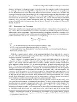
FIGURE 36.5 Dishing and erosion in copper CMP process. (From Ouma, D., Modeling of chemical–
mechanical polishing for dielectric planarization, Ph.D. Dissertation, Department of Electric Engineering and
Computer Science, MIT, Cambridge, 1998.)
transforms (FFTs) for computational efficiency, and (3) the use of layout masks with step densities
that facilitate the determin a tion of the ch aracteristic length (defined as the planarizatio n length) of
the elliptic function by introducing large abrupt post-CMP thickness variations.
36.3.3 COPPER CMP MODELING
Unlike oxide CMP, which involves the removal of only oxide material, the copper CMP involves
simultaneous polishing of three materials: copper, dielectric (oxide), and barrier. Barrier is a very
thin layer (Tan, Ti, etc.) that preventsthe copper from diffusing into the dielectric. The goal in copper
CMP is to remove the excess copper (also called overburden copper) and to polish the barrier on top
of the dielectric regions isolating the adjacent interconnect lines. This is required to preventelectrical
connection between adjacent interconnect lines. Owing to the heterogeneous nature of copper CMP,
a specific set of process parameters as well as a consumable set are required to achieve the p articular
RR for each corresponding material [68].
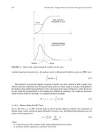
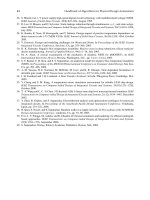
Two major defects caused b y copper CMP are pattern-dependent problems of metal dishing and

dielectric erosion as shown in Figure 36.6. If the height of the copper in the trench is lower than the
height of the neighboring dielectric, then dishing is positive otherwise it is negative. On the other
Dishing
Dielectric
Copper
Erosion
Pre-CMP
dielectric level
FIGURE 36.6 Dishing and erosion. (From Tugbawa, T., Chip-Scale modeling of pattern dependencies in
copper chemical–mechanical polishing processes, Ph.D. Dissertation, Department of Electrical Engineering
and Computer Science, MIT, Cambridge, MA, 2002.)
Alpert/Handbook of Algorithms for Physical Design Automation AU7242_C036 Finals Page 744 10-10-2008 #9
744 Handbook of Algorithms for Physical Design Automation
Field region Field regionRecess
Dielectric Copper
FIGURE 36.7 Definition of recess. (From Tugbawa, T., Chip-Scale modeling of pattern dependencies in
copper chemical–mechanical polishing processes, Ph.D. Dissertation, Department of Electrical Engineering
and Computer Science, MI T, Cambridge, MA, 2002.)
hand, dielectric erosion is always positive due to the loss of dielectric thickness during the CMP
process. The sum of dishing and erosion gives the copper thickness loss (also known as the copper
thinning) during CMP [68].
∗
Another p attern-dependent defect occurring during copper planarization is r ecess. Recess of a
copper interconnect line is equivalent to the dishing of that line. However, the recess of the dielectric
within an array of interconnect lines is the difference between the d ielectric height at a location
within the array and the height of surrounding dielectric fields as shown in Figure 36.7 [68].
The goal in copper CMP is to remove the excess copper and the unwanted barrier layer. Ideally,
this process should be fast without incurring extra dishing, erosion, or other defects. Owing to
heterogeneous nature of copper CMP, d ifferent materials are polished simultaneously. Initially, only
overburden copper is polished followed by the polishing of both copper and barrier film. Finally,

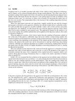
copper, barrier, and dielectric are polished at the same time. As stated in Ref. [68], to model copper
CMP process three stages of polish are identified: excess copper removal, barrier film removal, and
overpolish stage, as shown in Figure 36.8. In the excess copper removal stage, the evolution of the
Stage 1
Stage 3
Bulk
copper
removal
Barrier
removal
Overpolish
Oxide erosion
Cu dishing
Stage 2
FIGURE 36.8 Three intrinsic stages in copper CMP processes. (From Tugbawa, T., Chip-Scale modeling of
pattern dependencies in copper chemical–mechanical polishing processes, Ph.D. Dissertation, Department of
Electrical Engineering and Computer Science, MIT, Cambridge, MA, 2002.)
∗
In the published literature, erosion is sometimes referenced to the height of a neighboring field dielectric region, and a
separate field dielectric loss parameter is then specified. In Ref. [68], a single dielectric erosion term is used to r e present
dielectric loss.
Alpert/Handbook of Algorithms for Physical Design Automation AU7242_C036 Finals Page 745 10-10-2008 #10
CMP Fill Synthesis: A Survey of Recent Studies 745
copper thickness profile across the chip and the time it takes to remove the excess copper are of
interest. The time to polish the overburden copper varies across the die depending on the pattern
density at the location of interest.
In the second stage, copper and barrier film are polished simultaneously. The time to clear the
barrier film, as well as the dishing that results when barrier is removed at any location on the die, is
of interest. Due to process variation and deposited copper thickness variation across the wafer and
different pattern densities across the die, the RRs of the three materials (copper,barrier, and dielectric)

are d ifferent. This difference in RRs results in different polish times across the wafer for each stage.
For example, by the time the excess copper and barrier are cleared at a point on the die, they might
have already been cleared at another point. Hence, some points on the die are overpolished. In copper
CMP, overpolishingis defined as polishing beyond the time it takes to removethe overburden copper
and barrier at any spatial location. During the overpolishing stage, the dielectric is eroded [68].
In addition, the dishing that might have started during the barrier clearing stage can worsen
during overpolishing. This overpolishing is identified as the third intrinsic stage in the copper CMP
process. The dishing and erosion that occur during this stage are of interest. In computing the amount
of dishing during the overpolish stage, the dishing that occurs during the barrier clearing stage is
used as an initial condition. It is important to note that the term overpolishing is used loosely in the
CMP literature, and in the CMP industry [68].
∗
36.3.4 STI CMP MODELING
Shallow trench isolation is the isolation technique of choice in CMOS technologies. In STI, trenches
are etched in silicon substrate and filled with silicon dioxide to electrically separate active devices
[31]. The previously used isolationtechnique,LOCOS(local oxidationof silicon), suffers from lateral
growththat causes the isolation region to widen beyond the etched spaces. This lowers the integration
density. It also complicates device fabrication and introduces device functionality problems suc h as
high parasitic capacitances [47].
As describe d by Lee [36], the typical STI process flow initially involves growinga thin pad ox ide,
and then depositing a blanket nitride film on a raw silicon wafer. The isolation trenches ar e etched
such that the desired trench depth (i.e., depth from silicon surface) is achieved. The CMP process is
used to polish off the overburden dielectric down to the underlying nitride, where the nitride serves
as a polishing stop layer. After CMP, the nitr ide layer is then removed via etch, resultin g in active
areas surrounded by field trenches. A typical STI p rocess flow is shown in Figure 36.9.
Lee [36] identifies two major phases in STI CMP process. The first phase is the polish of
overburden oxide. The second phase is the overpolish into the nitride layer. The second phase is due
to the different pattern densities across the die, for example, CMP pad contacts the nitride layer at
different locations at different times. The first phase can be further broken down into two subphases.
The first subphase happens between the start of the polish and before the CMP pad contacts the

down areas (i.e., areas with lower height than their surroundings). The second subphase occurs from
the time CMP pad contacts the down areas until the up area overburden oxide has been completely
cleared to nitride.
The first subphase has a homogeneous nature in that only one material is being polished at each
moment. Reference [36] uses RR diagram to represent the polish of a single material. In this analysis,
the assumption is that the initial starting point is a spatial location on the dielectric layer with a fixed
step height. The feature densities for each poin t vary depending on the location on the die. Thus,
any spatial location with a fixed effective pattern density can be expressed using a RR diagram.
Figure 36.10 shows the RR diagram for phase one. For a significantly large step height, the CMP pad
only contacts the up areas, and the down area RR is zero. This is the first subphase denoted as phase
1A as shown in the figure. The up areas polish at a patterned RR, K/ρ, as shown on the RR diagram.
∗
In the CMP industry, overpolishing means polishing beyond the endpoint time.
Alpert/Handbook of Algorithms for Physical Design Automation AU7242_C036 Finals Page 746 10-10-2008 #11
746 Handbook of Algorithms for Physical Design Automation
Raw silicon wafer
Silicon wafer
Silicon wafer
Silicon wafer
Silicon wafer
Silicon wafer
Silicon wafer
Nitride removal
Active area
Field region
SiO
2
Nitride/pad oxide
z
0

T
Deposit nitride/oxide stack
Typical deposition
nitride 1500 Å
Etch isolation trenches
Typical trench depth 5000 Å
(does not include nitride/oxide stack)
Deposit dielectric
(SiO
2
oxide)
Typical deposition
z
0
= 9000 Å
CMP to remove
overburden oxide
FIGURE 36.9 Typical STI process. (From Lee, B., Modeling for chemical–mechanical polishing for shal-
low trench isolation, Ph.D. Dissertation, Department of Electrical Engineering and Computer Science, MIT,
Cambridge, MA, 2002.)
RR
K
0
Phase 1A
Phase 1APhase 1B
Phase 1B
Up area RR
Down area RR
h
c

Step height (H)
K
r
_
CMP pad
CMP pad
Oxide
Oxide
Phase 1A indicates polish before the CMP pad contacts the down areas.
Phase 1B indicates polish after down area has been initially contacted.
FIGURE 36.10 RR diagrams for STI CMP polish (oxide ov erburden phase). (From Lee, B., Modeling
for chemical–mechanical polishing for shallow trench isolation, Ph.D. Dissertation, Department of Electrical
Engineering a nd Computer Science, MIT, Cambridge, MA, 2002.)
Alpert/Handbook of Algorithms for Physical Design Automation AU7242_C036 Finals Page 747 10-10-2008 #12
CMP Fill Synthesis: A Survey of Recent Studies 747
RR
P
RR
P
Nitride
Slope K
P
nit
Slope K
P
ox
Oxide
FIGURE 36.11 RR versus pressure, for oxide and nitride. (From Lee, B., Modeling for chemical–mechanical
polishing for shallow trench i solation, Ph.D. Dissertation, Department of Electrical Engineering a nd Computer
Science, MIT, Cambridge, MA, 2002.)

As CMP process progresses, the step height reduces and eventually the polishing pad contacts the
down areas. This is when the second subphase starts, denoted as phase 1B in the figure. The up and
down RRs linearly approach each other until the step height is zero, after which the entire oxide film
is polished at the blanket oxide RR K [36].
Owing to heterogeneousnature of thesecondSTI CMP phase, a different removal diagramis used
to express the polish of the two separate materials of silicon dioxide and silicon nitride. Figure 36.11
shows the two RR versus pressure curves for n itride and oxide. Assuming a Prestonian relationship,
these are linear curves [36].
Dishing and erosion equations can be derived from the amount removal equations. These
equations are more useful because it is the dishing and erosion phenomenon that is of most inter-
est in STI CMP. The d ishing and erosion equations are also more useful because they isolate key
model parameters, making simpler equations from which to extract out model parameters. Dishing
is simply the step height as a function of time and erosion can be computed as the amount of nitride
removed.Therefore,dishing and erosion can be fully specified and predicted if the phase 1 and phase
2 STI CMP model parameters are known. These model p arameters are characteristic of a given CMP
process (tool, consumable set, etc.), and the model equations can be used to predict dishing and
erosion on wafers patterned with arbitrary layouts that are subjected to a specific characterized CMP
process [36]. In Section 36.4, density analysis methods are introduced. To asses the post-CMP effect,
the pattern density parameter must be computed.
36.4 DENSITY ANALYSIS METHODS
Traditionally, only foundries have performed the postprocessing needed to achieve pattern density
uniformity using insertion “filling” or partial deletion “slotting” of features in the layout [26]. How-
ever, layout pattern density must be calculated before addressing the filling or slotting problem.
Regions that are violating the lower and upper area density bounds are identified using density
analysis methods. Kahng et al. [26] present three density analysis approaches with different time
complexities all using the following density analysis problem formulation:
Extremal-density window analysis. Given a fixed window size w and a set of k disjoint rectangles in
an n × n layout region, find an extremal-density w ×w window in the layout.
∗
∗

Borrowing the terminology from Ref. [26], an extremal-de nsity window is a window with either maximum or minimum
density over all the windows throughout the layout.
Alpert/Handbook of Algorithms for Physical Design Automation AU7242_C036 Finals Page 748 10-10-2008 #13
748 Handbook of Algorithms for Physical Design Automation
Tile
Windows
FIGURE 36.12 Layout is partitioned by r
2
(r = 4) fixed dissections into
nr
w
×
nr
w
tiles. Each w × w
window (light gray) consists of r
2
tiles. A pair of windows from different dissections may overlap.
(Kahng, A.B., Robins, G., Singh, A., and Zehikovsky, A., Proceedings of IEEE International Confer ence
on VLSI Design, 1999.)
36.4.1 FIXED-DISSECTION REGIME
To verify (or enforce) upper and lower d ensity bounds for w × w windows, a very practical method
is to check (or enforce) these constraints only for w × w windows of a fixed dissection of the
layout into
w
r
×
w
r
tiles, that is, the set of windows having top-left corners at points (i ·

w
r
, j ·
w
r
), for
i, j = 0, 1, , r(
n
w
− 1), as shown in Figure 36.12. Here r is an integer divisor of w.
To analyze all the eligible w ×w windows takes a significant amount of time, while the analysis
of fixed dissections can be done much faster. Simply an array of
n
w
×
n
w
counters will be associated
with all the dissection windows, and then for each rectangle R the counters of windows intersecting
R will be incremented by the area of intersection. In general, the above procedure must be repeated
r
2
times to check all the (r ·
n
w
)
2
windows [26].
36.4.2 MULTILEVEL DENSITY ANALYSIS
Even though the fixed dissection analysis can be performed quickly, it can underestimate the max-

imum floating-window density worst case.
∗
Kahng et al. [28] propose a new multilevel density
analysis approach that, as opposed to the techniques presented in Refs. [26,27], has the efficiency
of the fixed dissection analysis without sacrificing the accuracy for the floating window worst-case
analysis. The multilevel density analysis is based on the following simple observation.
Observation. Given a f ixed r-dissection, any arbitrary floating w × w window will contain some
shrunk w(1 − 1/r) × w(1 − 1/r) window of the fixed r-dissection, and will be contained in
some bloated w(1 +1/r) ×w(1 + 1/r) window of the fixed r-dissection as shown in Figure 36.13.
The first implication of the above observation is that the floating window area can be upper
bounded by the area of bloated windows, and lower bounded by the area of shrunk windows. A fixed
∗
In general, when all the eligible windo ws are being examined and filled, it is referred to as the floating window regime.
Alpert/Handbook of Algorithms for Physical Design Automation AU7242_C036 Finals Page 749 10-10-2008 #14
CMP Fill Synthesis: A Survey of Recent Studies 749
Fixed dissection
window
Floating window W
Shrunk fixed
dissection window
Bloated fixed
dissection window
Tile
FIGURE 36.13 Any floating w × w window W always contains a shrunk (r − 1) × (r − 1) window of a
fixed r-dissection, and is always covered by a bloated (r + 1) × (r + 1) window of the fixed r-dissection.
(Kahng, A. B., Robins, G., Singh, A., and Zehikovsky, A., Proceedings of IEEE Asia and South Pacific Design
Automation Conference, 1999.)
r-dissection regime can be recursively subdivided into smaller dissections until the number of tiles
in each dissection is small. Then the floating density analysis can be applied without significant
runtime complexity. In addition, the recursion can be term inated once the floating density analysis

is within some user-defined criteria, say ε = 1 percent [28]. In this subsection, different density
analysis approaches proposed by the authors of Refs. [26–28] have been presented.
36.5 CMP FILL SYNTHESIS METHODS
Layout density problem includes two stages: density analysis and fill synthesis. Having presented
the different approachesproposed for the density analysis stage, in this section the techniques used in
fill synthesis will be reviewed. The first fill synthesis approach proposed by Ref. [26] was basically
to first sort all the wires by rows, and within each row sort them by the coordinates of their leftmost
starting points. Then, for each row, from left to right, metal fill would be placed in the space between
the wires as shown in Figure 36.14. This simple method is based on scanline algorithm principles
and is applicable to only wiring-type layouts. Reference [26] also proposes a simple technique for
slotting. However, due to the reliability issues arising from slotting (i.e., change in current density
due to change in wire cross section) it was not studied further, and the main focus of research is on fill
insertion approaches. In the following four subsections, in Section 36.5.1, different density-driven
problem formulations are presented. In Section 36.5.2, the model-based fill synthesis approach is
introduced. In Section 36.5.3 the impact of CMP fill on cir cuit performance is investigated. An d in
Section 36.5.4, a new fill insertion method to be used in STI process is discussed.
36.5.1 DENSITY-DRIVEN FILL SYNTHESIS
The following notation and definitions are used in defining the filling problem as described in
Ref. [27].
Alpert/Handbook of Algorithms for Physical Design Automation AU7242_C036 Finals Page 750 10-10-2008 #15
750 Handbook of Algorithms for Physical Design Automation
(a)
(b)
FIGURE 36.14 (a) Example of a wiring-type layout and (b) a corresponding fill solution. (Kahng, A. B.,
Robins, G., Singh, A., Wang, H ., and Zelikovsky, A., Pr oceedings of ACM/IEEE International Symposium on
Physical Design, 1998.)
• Input is a layout consisting of rectangular geometries, with all sides having length as a
multiple of c (min imum feature width, spacing).
• n ≡side of thelayout region. If the layoutregionis theentiredie, nmight be about 50, 000·c.
• w ≡ fixed window size. The window is the moving square area over which the layout

density rule applies.
• k ≡ layout complexity, number of input rectangles.
• U ≡area density upper bound, expressed as a real number 0 < U < 1. Each w ×w region
of the layout must contain total area of features ≤ U · w
2
.
• B ≡ buffer distance. Fill geometries cannot be introduced within distance B of any layout
feature.
• slack (W) ≡ slack of a given w × w window W. Slack (W) is the maximum amount of fill
area that can be introduced into W.
Using the above no tation and definition the filling problem is stated as follows [27]:
Filling problem. Given a design rule-correct layout geometry of k disjoint rectilinear rectangles in
an n ×n layout region, minimum feature size c, window size w < n, buffer distance B, and area (or
perimeter) density lower bound L and upper bound U, add fill geometries to create a filled layout
that satisfies the following conditions:
1. Circuit functionality and design rule-correctness are preserved.
2. No fill geometry is within distance B of any layout feature.
3. No fill is added into any window that has density ≥U in the original layout.
4. For any window that has density <U in the o riginal layout, the filled layout density is ≥L
and ≤U.
5. Minimum window density in the filled layout is maximized.
Condition (5) corresponds to the so-called min-variation objective. This constraint minimizes the
difference between minimum and maximum window density in the filled layout. However, adding
fill will impact circuit performance by changing the total and coupling interconnect capacitances. To
attack this problem, another objective called min-fill, has been added to the previous min-variation
objective, which deletes as much previously inserted fill as possible, while preserving a minimum
window density of no less than the lower bound L.
Alpert/Handbook of Algorithms for Physical Design Automation AU7242_C036 Finals Page 751 10-10-2008 #16
CMP Fill Synthesis: A Survey of Recent Studies 751
36.5.1.1 LP-Based and Monte-Carlo-Based Methods

Kahng et al. [27] propose the first min-variation formulation using a linear programming (LP)
approach. In a fixed r-dissection regime, for any given tile T = T
ij
, i, j = 1, ,
nr
w
, the total feature
area inside T and the maximum fill amount that can be placed within T without violating the density
upper bound U in any window containing T are denoted as area (T ) and slack (T), respectively. The
following is the filling problem as described in Ref. [27].
Filling problem for fixed r-dissection. Suppose a fixed r-dissection of the layout with tiles of size
w
r
×
w
r
,aswellasanarea(T ) and slack (T) for each tile in the dissection. Then, for each tile T
ij
,the
total fill pattern area p
ij
= p(T
ij
) to be added to T
ij
must satisfy
0 ≤ p
ij
≤ slack(T
ij

)
and

T
ij
∈W
p
ij
≤ max{U · w
2
− area(W),0} (36.3)
for any fixed dissection w ×w window W.
Then, the min-variation fo rmulation seeks to maximize the minimum window density:
Maximize

min
ij
(area(T
ij
) + p
ij
)

The linear programming approach seeks the optimum fill area p(T
ij
) to be inserted into each tile
T
ij
. Recall that the fill area p(T
ij

) cannot exceed slack (T
ij
), which is th e area available for filling inside
the tile T
ij
computed during density analysis. The first LP for the min-variation objective [27,29] is
Maximize M
subject to
0 ≤ p(T
ij
) ≤ slack(T
ij
)
M ≤ ρ(M
ij
) ≤ Ui, j = 1, ,
nr
w
− 1
An important step in the above LP approach is to deter mine slack values. To calculate the total
area of all the possible overlappingrectangles the approach of measure of union of rectangles sweep-
line-based technique [53] has been used. In a follow up work by the authors in Ref. [68], the fill
placement problem was described by the following LP formulation:
Minimize

i,j
p(T
ij
)
subject to

0 ≤ p(T
ij
) ≤ slack(T
ij
)
L ≤ ρ(M
ij
) ≤ Ui, j = 1, ,
nr
w
− 1
Reference [68] also proposes a variant LP approach, that manufacturability does not require the
extreme min-variation formulation, that is, given a target window density M, a variability budget
ε must be minimized: