Handbook of algorithms for physical design automation part 91 pps

Alpert/Handbook of Algorithms for Physical Design Automation AU7242_C042 Finals Page 882 23-9-2008 #3
882 Handbook of Algorithms for Physical Design Automation
microprocessors are presented to illustrate h ow the basic techniques described in this ch apter are
applied in practice.
42.1 METRICS FOR CLOCK NETWORK DESIGN
Unlike other signals that carry data information, the clock signal in edge-triggered circuits carry
timing informationby the signal transitions(i.e., edges). Therefore, the metrics used in clock network
design are different from those for general signal net design, and these are discussed in the remainder
of this section.
42.1.1 SKEW
Clock skew refers to the spatial variation in the arrival time of a clock transition. The clock skew
between two points i and j on a chip is defined as t
i
− t
j
,wheret
i
and t
j
are the clock arrival time
to point i and point j, respectively. The clock skew of a chip is defined as the maximum clock
skew between any two clocked elements on the chip. In general, clock skew forces designers to be
conservative and use a longer clock period, that is, a lower clockfrequency, for the design (unlessboth
the clock network and the circuit are specially designed to take advantage of clock skew as described
in Section 42.4). Therefore, clock networks with zero skew are most desirable. However, because of
static mismatches in the clock paths and clock loads, clock skew is nonzero in practice, and hence
skew minimization is always one of the most important objectives in clock network design. Skew
can be effectively minimized in both physical design and circuit design stages. Skew minimization
approaches in physical design stage are discussed in this chapter. Deskewing techniques in circuit
design stage will be illustrated by several examples in Chapter 43.
Jitter is anoth er measure of the variation in the arrival time of a clock transition. Specifically, it

refers to the temporal variation of the clock period at a given point on the chip. Like skew, it is an
important metric to the quality of the clock signal because it also forces designers to be conservative
and usea longer clock period. The structureof the clock networkhas insignificant effect onjitter.Jitter
is caused by delay variation in clock buffer due to power supply noise and temperature fluctuation,
influence o f substrate/power supply noise to the clock generator, capacitive coupling between clock
and adjacent signal wires, and data-dependent nature of load capacitance of latch/register [1]. It is
more effectively minimized by the d esign of other components like power supply network and clock
generator. Therefore, it is typically not considered during clock network design.
42.1.2 TRANSITION TIME
The transition time is usually defined as the time for a signal to switch between 20 and 80 percent of
the supply voltage.
∗
This corresponds to the rise time for the rising transition, and the fall time for
the falling transition. The reciprocal of the transition time is called the slew rate.
†
Slow transitions could potentially cause large skew and jitter values in the presence of process
variations or noise. Transition timesalso need tobe substantially less thanthe clock periodto allow the
clock to achieve a rail-to-rail transition, to provide adequate noise immunity. Another motivation for
sharp transition times is that they limit the short-circuit power, which is roughlyproportional to input
transition time [2], in the clock network. However, to reduce transition time, larger or mo re buffers
are normally required, which would increase power consumption, layout congestion, and process
variations. In practice, transition times are bounded rather than minimized in clock network design.
∗
Definitions as switching time between 10 and 90 percent, and between 30 and 70 percent are also common.
†
However, in common u sage, the term slew rate is often used to mean tr ansition time r ather than its reciprocal.
Alpert/Handbook of Algorithms for Physical Design Automation AU7242_C042 Finals Page 883 23-9-2008 #4
Clock Network Design: Basics 883
42.1.3 PHASE DELAY
Phase delay (or latency) is defined as the m aximum delay from the clock generator to any clock

terminal. It is important to realize that because the clock is a periodic signal, the absolute delay
from the clock generator to a clock terminal is not important. However, it has been observed that
the shorter the phase delay, the more robust the clock network will generally be [3]. Therefore, the
phase delay can be used as a simple albeit indirect criterion in clock network design.
42.1.4 AREA
The clock network is a huge structure driving a large number of widely distributed terminals. It
consists of a large number of wire segments, many of which are long and wide. Hence the clock
network utilizes a significant wire area. For example, it con su mes 3 percent of the total available
metals 3 and 4 [4]. Moreover, because the clock network is sensitive to noise, it is usually shielded
and hence uses even more wire resources. In addition, typically, a lot o f possibly large buffers are
inserted in the clock network. Those buffers could occupy a significant device area. It is important
to minimize both wire area and device area in clock network design.
42.1.5 POWER
Because of battery life concern in portable electronic devices and heat dissipation problem in high-
performance ICs, power consumption is a very important design consideration in recent years. The
clock signal switches twice every cycle. Whenever it switches, the huge capacitance associated
with the wires and devices of the c lock network needs to be charged or discharged. Therefore,
clock distribution is a significant component of total power consumption. The clock distribution and
generation circuitry is known to consume up to 40 percent and 36 percent of the total power budget
of high-performance [4] and embedded [5] microprocessors, respectively. However, a significant
portion of the clock power is consumed in the input capacitance of the clocked elements [3,6].
Unless large amounts of local clock g ating is done, as is typical in high-performance designs, this
portion of power cannot be reduced by modifying the clock network.
42.1.6 SKEW SENSITIVITY TO PROCESS VARIATIONS
If the manufacturing process is ideal, a careful clock network design can eliminate any clock skew.
However,with reductions in thefeature sizesof VLSI processes, manufacturing variationsare becom-
ing increasingly significant. These variations are the major causes of clock skew in modern designs,
as designers usually can keep the systematic skew under nominal process parameters low. As a
design goal, it is important not only to minimize metrics such as the skew but also to minimize their
sensitivity to process variations.

42.2 CLOCK NETWORKS WITH TREE STRUCTURES
A common and simple approach to distribute the clock is to use a tree structure. The most basic tree
structure is the H-tree as shown in Figure 42.1, and it is obtained by recursively drawing H-shapes
at the leaf nodes. With enough recursions, the H-tree can distribute a clock from the center to within
an arbitrarily short distance of every point on the chip.
If all clock terminals have the same load and are arranged in a regular array as in Figure 42.1, and
if there is no process variation, the H-tree will have zero skew. However, the clock loads are almost
always irregularly arranged all over the chip. To handle the irregularity, algorithms that produce
generalized H-tree structures are presented in Sections 42.2.1 through 42.2.4. Wire sizing and buffer
insertion in clock trees are discussed in Section 4 2.2.5.
As a notational matter, we point out that Manha ttan distances and rectilinear rou ting are assumed
throughout this chapter. However, for simplicity, nonrectilinear segments are drawn in most figures
Alpert/Handbook of Algorithms for Physical Design Automation AU7242_C042 Finals Page 884 23-9-2008 #5
884 Handbook of Algorithms for Physical Design Automation
AB
Source
Terminal
FIGURE 42.1 Clock network for 64 terminals with H-tree structure.
(e.g., Figure 42.2). Each nonrectilinear segment can be replaced by a set of two (or more) rectilinear
segments in an actual implementation.
42.2.1 METHOD OF MEANS AND MEDIANS
Jackson et al.[7] proposed analgorithm called themethod ofmeans andmedians (MMM)to construct
a clock tree for a set of arbitrarily distributed terminals. The algorithm takes a top-down recursive
approach, a recursive step of wh ich is illustrated in Figure 42.2. In each step, the set of terminals is
partitioned acco rding to either the x-ory-coordinate into two subsets about the median coordinate of
the set. Note that the number of terminals in the two subsets may be equal, if the number of nodes is
even, or may differ by one otherwise. Then the center of mass (i.e., mean coordinate) of the entire set
is connected to both centers of mass of the two subsets. The partitionin g directio n at each recursive
level is determined by an one level look-ahead technique in which both x-then-y partitioning and
y-then-x partitioning are attempted, and the one that minimizes skew between its current endpoints

is chosen. The clock trees for the subsets are recursively constructed until there is only one terminal
in each subset. The time complexity of MMM is O(n log n),wheren is the number of terminals.
42.2.2 GEOMETRIC MATCHING ALGORITHM
The geometric matching algorithm (GMA) proposed by Kahng et al. [8] solves the same prob-
lem formulation as the MMM algorithm, but takes a bottom-up recursive approach. A geometric
Center of mass
of subset 2
Subset 2
Center of mass
of subset 1
Center of mass
of whole set
Subset 1
Median of whole set
in x direction
FIGURE 42.2 Recursive step of the MMM algorithm. The set is partitioned according to x-coordinate.
Alpert/Handbook of Algorithms for Physical Design Automation AU7242_C042 Finals Page 885 23-9-2008 #6
Clock Network Design: Basics 885
(a) (b) (c)
FIGURE 42.3 Recursive steps of t he GMA algorithm. Seven terminals are merged into four subtrees in (a),
then two subtrees in (b), and finally one subtree in (c).
matching of a set of k points is a set of k/2 line segments connecting the points, with no two
line segments connecting to the same point. The cost of the g eometric matching is the sum of the
lengths of its line segments. The GMA is illustrated in Figure 42.3. In each recursive step, a set of
k path-length-balanced subtrees are g iven. (At the beginning, each terminal is a subtree by itself.)
The subtrees are merged by finding a minimum-cost matching of their tapping points (i.e., roots) to
form k/2 new subtrees. The tapping point of each new subtree is chosen to be the b alance point
that minimizes the maximu m difference in path lengths to the leaves of the subtree. The resulting
set of subtrees (including the k/2 new ones and potentially one unmatched subtree when k is odd)
will be recursively matched until a single path-length-balanced tree is obtained.

In some cases, it is impossible to find a balance point such that the path lengths to all leaves are
exactly the same. For example, in Figure 42.4a, if l
1
+l < l
2
, then the best balance point is node A but
the path lengths to leaves are still not completely balanced . For those cases, a H-flipping operation
as shown in Figure 42.4b can be applied to reduce the skew.
If using optimal matching algorithm in planar geometry, the time complexity of GMA is
O(n
2.5
log n),wheren is the number of terminals. Faster nonoptimal matching heuristics can also be
used to speed up the algorithm. It was experimentally shown in Ref. [8] that the trees generated by
GMA are better in wirelength and skew than those by MMM.
42.2.3 EXACT ZERO-SKEW ALGORITHM
Both the MMM algorithm and GMA assume the delay is linear to the path length, and then focus
on balancing of path lengths. For high-performance designs with tight skew constraints, algorithms
based on more accurate delay models are desirable. Tsay [9] presented an algorithm that produces
clock trees withexact zero skew according to the Elmoredelay model [10].Like GMA, this algorithm
recursively merges subtrees in a bottom-up manner. However, it assumes that a tree topology, which
determines the pairing up of subtrees, is given. It addresses the problem of finding the tapping points
precisely so that the merged trees have zero skew.
Suppose two zero-skew subtrees are merged by a wire of length l as shown in Figure 42.5a.
The wire is divided by the tapping point into two segments of length xl and (1 − x)l, respectively.
By representing each subtree by a lumped delay model and each segment by a π-model, we can
transform the circuit into an equivalent RC tree as shown in Figure 42.5b.
(a)
(b)
H-flipping
A

l
l
2
l
1
FIGURE 42.4 H-flipping operation for further skew minimization.
Alpert/Handbook of Algorithms for Physical Design Automation AU7242_C042 Finals Page 886 23-9-2008 #7
886 Handbook of Algorithms for Physical Design Automation
(b)
(a)
Tapping point
Subtree 2
Subtree 1
xl
(1Ϫx)l
Subtree 2
Subtree 1
t
2
t
1
r
1
r
2
C
1
c
1
/2 c

1
/2 c
2
/2 c
2
/2
C
2
FIGURE 42.5 Zero-skew merge of two subtrees.
To ensurethe delay fromthe tapping pointto leaf nodesof both subtreesto beequal,it requiresthat
r
1
(
c
1
/2 +C
1
)
+ t
1
= r
2
(
c
2
/2 +C
2
)
+ t
2

(42.1)
Let α be the wire resistance per unit length and β be the wire capacitance per unit length. Then,
r
1
= αxl, r
2
= α(1 − x)l, c
1
= βxl,andc
2
= β(1 − x)l. Hence, after solving Equation 42.1, we
find the zero-skew condition to be
x =
(
t
2
− t
1
)
+ αl
(
βl/2 + C
2
)
αl
(
βl + C
1
+ C
2

)
If 0 ≤ x ≤ 1, it indicates that the delay can be balanced by setting the tapping point som ewhere
along the segment. On the other hand, if x < 0orx > 1, it implies the two subtrees are too much out
of balance and extra delay needs to b e introduced through wire elongation, which is commonly done
by snaking. Without loss of generality, consider the case x < 0. For this case, the tapping point has
to be at the root of subtree 1 and the segment connecting subtree 1 to subtree 2 has to be elongated.
Assume the length of the elongated segment is l

. To balance the delay,
t
1
= t
2
+ αl


βl

/2 +C
2

or
l

=

(
αC
2
)

2
+ 2αβ
(
t
1
− t
2
)
− αC
2
αβ
Similarly, for the case x > 1, the tapping point should be at the root of subtree 2, and
l

=

(
αC
1
)
2
+ 2αβ
(
t
2
− t
1
)
− αC
1

αβ
Alpert/Handbook of Algorithms for Physical Design Automation AU7242_C042 Finals Page 887 23-9-2008 #8
Clock Network Design: Basics 887
(a) (b)
E
A
B
F
D
C
G
E
A
B
G
C
D
F
FIGURE 42.6 Two different ways to construct a zero-skew clock tree f or terminals A–D. The connection EF
in (b) is much shorter than the one in ( a).
42.2.4 DEFERRED MERGE EMBEDDING
In the exact zero-skew algorithm in Section 42.2.3, there are many possible ways to route the
connection between each pair of tapping points. As shown in Figure 42.6, the routing will determine
the location of the tapping point, and hence the wirelength of the connection at the next higher level.
In Ref. [9], it was suggested that a few possible wiring patterns (e.g., two one-bend connections)
may be constructed and the one which gives a shorter length at the next level is picked.
In general, the problem is to embed any given connection topology to create a zero-skew clock
tree while minimizin g total wirelength. This problem can be solved in linear time by the defer red
merge embedding (DME) method independently proposed by Edahiro [11], Chao et al. [12], and
Boese and Kahng [13]. The DME algorithm consists of two phases. First, a bottom-up phase finds

a line segment called the merging segment, ms(v), to represent all possible placement locations for
each tapping point v. Then, a top-down phase resolves the exact location for each tapping point.
We use the example in Figure 42.6 to explain how to find the merging segments in the bottom-up
phase. The steps are illustrated in Figure 42.7. Consider the tapping point E. The distances d
AE
from
A to E and d
BE
from B to E that balance the delay according to some delay model are first computed.
The algorithm to compute the distances depends on the delay model used. For example, for Elmore
delay model, Tsay’s algorithm[9] can be applied. Then we set ms(E) to bethe set of all points within
a distance d
AE
from A and within a distance d
BE
from B. ms(F) can be found similarly. Next, consider
the tapping point G. The least possible length of the connection between E and F is the minimum
distance between any point in ms(E) and any point in ms(F). Based on this length, we can compute
the d istances d
EG
from E to G and d
FG
from F to G that balance the delay. Finally, we set ms(G) to
be the set of all points within a distance d
EG
from some point in ms(E) and within a distance d
FG
from some point in ms(F).
A Manhattan arc is defined to be a line segment, possibly of zero length, with slope +1or−1.
A crucial observationis that all merging segmentsare Manhattan arcs. To prove this observation,first

(a) (b)
d
AE
d
BE
d
CF
d
DF
ms(F )
ms(E )
C
A
D
B
d
EG
d
FG
A
D
B
C
ms(G )
ms(E )
ms(F )
FIGURE 42.7 Construction of merging segments in the bottom-phase of DME.
Alpert/Handbook of Algorithms for Physical Design Automation AU7242_C042 Finals Page 888 23-9-2008 #9
888 Handbook of Algorithms for Physical Design Automation
notice that the merging segment of a terminal is a single point and thus a Manhattan arc. Consider

the merge of two subtrees rooted at X and Y to form a tree rooted at Z such that both ms(X) and
ms(Y) are Manhattan arcs. Let l be the minimum distance between any point in ms(X) and any point
in ms(Y). l is the least possible length of the connection between X and Y. To balance the delay, we
compute d
XZ
and d
YZ
. There are two possible cases. The first case is d
XZ
+ d
YZ
= l. Note that both
the region within a distance d
XZ
from ms(X) and the region within a distance d
YZ
from ms(Y) are
tilted rectangles. Moreover, the two rectangles are touching each other as d
XZ
+ d
YZ
= l.ms(Z) is
set to the intersection of them and hence is a Manhattan arc. The second case is d
XZ
+ d
YZ
> l.In
this case, Z coincides with either X or Y, and wire is elongated to balance the delay. Without loss of
generality, assume Z coincides with X.Thenms(Z) is set to all points in ms(X) that are also within
a distance d

YZ
from ms(Y). Hence it is also a Manhattan arc. By induction, therefore, all merging
segments must be Manhattan arcs. Because of this observation, each merging segment can be found
in constant time. The whole bottom-up phase requires linear time.
For the top-down phase,the locations of tapping points are fixed in a top-down manner asfollows.
For the root r of the whole tree, its location is set to any point in ms(r). For any other tapping point
v, its location is set to any point in ms(v) that is within a distance d
vp
(determined in bottom-up
phase) from the location of v’s parent p. The top-down phase also takes linear time. Therefore, DME
is a linear time algorithm. It has been proved that for linear (i.e., path length) delay model, DME
produces zero-skew tree with optimal wirelength. However, it has also been shown that DME is not
optimal for Elmore delay model [13].
Instead of achieving zero skew, the DME algorithm can be extended to handle general skew
constraints. The extended DME algorithm has applications in clock skew scheduling (Section 42.4)
and process variation aware clock tree routing (Section 42.5).
42.2.5 WIRE WIDTH AND BUFFER CONSIDERATIONS IN CLOCK TREE
Wire resistance is a major concern for clock tree design in advanced process. If a clock wire is long
and narrow, it will have a very significant resistance. Together with the significant capacitive load of
the clock wires and terminals, this implies that the clock signal will have very long phase delay and
transition time. Note that this problem cannot be resolved merely by increasing the driving strength
(i.e., size) of the clock generator. Even though a strong clock generator can produce a sharp clock
signal at the source, the signal degrades rapidly as it is transmitted through the lossy clock wire.
One solution is to size up the width o f the clock wires as wire resistance is inversely proportional
to the wire width. Such a method must requir e a router to handle wires of varying widths, and also
requires appropriatesizing of the clock driversto meetthe delay andtransition time constraints under
an increased load for the stage.
Another solution is to insert buffers distributively in the clock tree: the basic concept is similar
to buffer insertion for signal lines, d iscussed elsewhere in this book. Buffers are effective in main-
taining the integrity of the clock signal by restoring degraded signals. Buffered clock trees generally

use smaller clock generator and narrower wires, and hence consume less power and area [14,15].
However,buffer delay is more sensitive to process variationsand power supply noise than wire delay.
Hence, buffered clock trees may have more skew and jitter. Moreover, clock tree design is typically
performed after placement so that clock terminals are fixed. Inserting the clock buffers into a placed
circuit may be difficult.
To reduce skew and skew sensitivity to process variations in buffered clock tree design, the
following guidelines are often followed:
• Buffered clock trees should have equal numbers of buffers in all source-to-sink paths
• At each buffered level, the buffers should have the same size
• At each buffered level, the buffers should have the same capacitive load and the same input
transition time (potentially by adjusting the width and length of the wires)
Alpert/Handbook of Algorithms for Physical Design Automation AU7242_C042 Finals Page 889 23-9-2008 #10
Clock Network Design: Basics 889
In practice,a mixed approachof wire width adjustmentand buffer insertionis typically used[16].
For example, Restle et al. [3] presented the clock n etwork design of six microprocessor chips. In all
these chips, the clock network consists of a series of buffered treelike networks driving a final set
of 16–64 sector buffers. Each sector buffer drives a tree network tunable by adjusting wire widths.
(The tunable trees finally drive a single clock grid, which is discussed in Section 42.3.1.)
42.3 CLOCK NETWORKS WITH NONTREE STRUCTURES
Although tree structures are relatively easy to design, a significant drawback associated with them
is that, in the presence of process variations, two physically nearby points that b elong to different
regions of the clock tree, may have a significant skew. For example, points A and B in Figure 42.1
may experience a large skew because the two paths from source to them are distinct and may not
match well with each other. This kind of local skew is particularly troublesome, because physically
nearby registers are likely to be connected by a combinational path. Therefore, the significant skew
can easily cause a hold time violation, which is especially costly as it cannot be fixed by slowing
down the clock frequency.In the following, several nontree structures are introduced. They are more
effective in reducing skew in a local region, but they consume more area and power.
42.3.1 GRID
A clock grid is amesh o f horizontaland vertical wires driven from the middle or edges. Typcially,the

mesh is fine enough to deliver the clock signal to within a short distance of every clocked element.
The skew minimization approach of grids is fundamentally different from that of trees. Grids try to
equalize delay of different points by connecting them together, whereas trees try to balance delay of
different points by carefully matching the characteristics of different paths.
As the grid connects nearby points directly, it is very effective in reducing local skew. Moreover,
its design is not as sensitive to the placement details as a tree structure, which makes late design
changes easier. On the other hand, for a tree-structured network, if a late design change significantly
alters the locations of the clocked elements or the values of the load capacitances, an entirely new
tree topology may be required. The main disadvantage of grids is that they consume a large amount
of wire resources and power. In addition, grids may have significant systematic skew between the
points closest to the drivers and the points furthest away. This problem can be illustrated by the clock
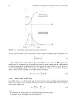
network design of the 300 MHz Alpha 21164 processor [17], where the clock signal generated at the
center of the chip is distributed to the left and right banks of final clock drivers (Figure 42.8a), which
then drive a grid. It is clear from the simulation results in Figure 42.8bthat the skews between points
near the left and right drivers and points further away are very significant (up to 90 ps). Therefore,
grids are rarely used by themselves. A balanced structure is usually employed to distribute the clock
globally to various places in the grid, as discussed in Section 42.3.3.
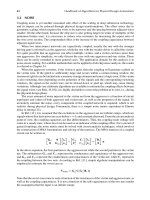
42.3.2 SPINE
The spine structure for clock distribution is shown in Figure 42.9. A clock spine is a long and
wide piece of wire running across the chip, which drives the clock signal through delay-matched
serpentine wires into each small group of clocked elements. This idea was first introduced by Lin
and Wong [18]. Typically, the clock signal is distributed from the clock generator to the spine by a
balanced buffered tree such that it arrives at many different points of the spine simultaneously. If the
load distribution induced by the serpentine wires on the spine is uniform, the spine has zero skew
everywhere. If the delays of the serpentine wires are perfectly matched, then the skew at the clocked
elements will also be zero.
Like grids, spines provide a stable structure that facilitates late design changes. Although this
structure does not make the clock as readily available as grids so that serpentine routing is required,
a serpentine is easy to design. To accommodatefor late d esign changes, each serpentine can be tuned
Alpert/Handbook of Algorithms for Physical Design Automation AU7242_C042 Finals Page 890 23-9-2008 #11

890 Handbook of Algorithms for Physical Design Automation
80
72
64
56
48
40
32
24
16
8
0
17
16
15
14
13
12
11
10
9
Y (mm)
8
7
6
5
4
3
2
1

0
0
1
2
3
4
5
6
7
X (mm)
8
9
10
11
12
13
14
15
16
17
(b)(a)
Clock drivers
Delay (ps)
FIGURE 42.8 Clock driver locations (a) and clock delay in Alpha 21164 (b). (Courtesy of Hewlett-Packard
Company.)
Spine 1
Spine 2
Delay-matched
serpentine routing
FIGURE 42.9 Clock distribution by spines with serpentine routing.

individually without affecting others. Moreover, clock gating is easy to be incorporated as each
serpentine can be gated separately. However, a system with many clocked elements may require a
lot of serpentine routes, which cause high area and power consumption. Like trees, spines also may
have large local skews between nearby elements driven by different serpentines.
Intel has used the spine structure in its Pentium processors. Details can be found in Chapter 43.
42.3.3 HYBRID
The tree structure is good atminimizing skew globally,while thegrid structure is effective in reducing
skew locally. To achieve low skew at both global and local levels, tree and grid can be combined to
form a hybrid structure. A practical approach is to use a balanced tree to distribute the clock signal
to a large number of points across the chip, and then a grid to connect these points together. As the
grid is driven in many points, the systematic skew problem of grid is resolved. Moreover, as the tree
sinks are shorted by grid segments, the local skew problem of tree is eliminated. In high-performance
Alpert/Handbook of Algorithms for Physical Design Automation AU7242_C042 Finals Page 891 23-9-2008 #12
Clock Network Design: Basics 891
Zero-skew
subtree 1
Zero-skew
subtree 2
Zero-skew
subtree 3
Zero-skew
subtree 4
Zero-skew mesh
Clock driver
or buffer
FIGURE 42.10 Clock network with a global mesh driving local trees.
design, the skew budget is too tight to be satisfied either by a pure tree or a pure grid approach. The
hybrid approach is a common alternative. In addition, like a grid, the hybrid network also provides
a stable structure that facilitates late design changes. The only drawback of this approach is power
and area cost even higher than a pure grid approach.

Many microprocessors have used a hybrid structure for clock distribution, and several of them
are discussed in Chapter 43. In particular, IBM has used the hybrid approach on a variety of micro-
processors including the Power4, PowerPC, and S/390 [3]. In the IBM designs, a primary buffered
H-tree drives 16–64 sector buffers arranged on the chip. Each sector buffer drives a smaller tree
network. Each tree can be tuned to accommodate nonuniformload capacitance by adjusting the wire
widths. Together, the tunable trees drive a global clock grid at up to 1024 points.
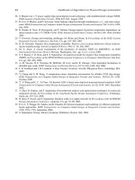
Su and Sapatnekar [19] proposed a different hybrid approach. In this mesh/tree approach, a
global zero-skew mesh is used to drive local zero-skew trees as shown in Figure 42.10. This idea
can be generalized to a multilevel structu re in which each subtree sink at a certain level is driving
another mesh with four subtrees at the next lower level.
To construct an one-levelmesh/tree clocknetwork, the sinks are first divided into four groupsand
a buffered tree is built for each group by any zero-skew tree construction algorithm (e.g., Tsay [9]).
Basedon thedelay anddownstreamcapacitanceof the fourtrees,a zero-skewmeshis thenconstructed
by adjusting the width of the eight mesh segments. Interestingly, they show that the problem of
minimizing the total segment area to achieve zero skew with respect to Elmore delay (by requiring
all four trees to meet a given target delay) can be formulated as a linear program of only four of the
segment width variables. A heuristic procedure is presented to iteratively set the target delay and
possibly elongate some segments until a feasible solution (with all segment widths within bounds)
is found. As a postprocessing step, wire width optimization under an accurate higher-order delay
metric is performed.
It is shown experimentally that clock networks by this hybrid mesh/tree approach are better in
skew, skew sensitivity, phase delay, and transition time than trees by Tsay’s algorithm. They are
also better in skew, phase delay, and transition time, and similar in area when comparing to the IBM
structures discussed above.
42.4 CLOCK SKEW SCHEDULING
The clock skew scheduling technique makes use of intentional nonzero clock skews to optimize
the performance of synchronous systems. The basic idea is to use clock skews to balance the slack
differencebetween combinational paths instead of achieving zero-skew clock arrival times. This idea
was first proposed by Fishburn [20].
Before presentingthe clock skew scheduling problem formulations, we first introduce the timing

constraints on clock signals. To avoid clock hazards, setup time constraints and hold time constraints
have to be satisfied by all source/destination register pairs in the system. Consider a pair of registers