Parallel Programming: for Multicore and Cluster Systems- P7 pptx

50 2 Parallel Computer Architecture
4
444
4
4
3
3
3
555
y
x
(0,0) (1,0) (2,0)
(0,1) (1,1) (2,1)
(0,2) (2,2)(1,2)
12
1
1
1
1
0
2
2
1
0
0
1
1
4
35 5 5
0
2

44 44 4
2
0
1
1
1
10
2
33
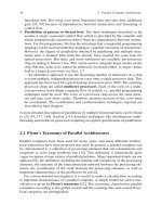
2D mesh with 3 x 3 nodes channel dependence graph
Fig. 2.21 3 ×3 mesh and corresponding channel dependence graph for XY routing
This is a contradiction, and thus no deadlock can occur. Each routing path selected
by XY routing consists of a sequence of links with increasing numbers. Each edge
in the channel dependence graph points to a link with a larger number than the
source link. Thus, there can be no cycles in the channel dependence graph. A similar
approach can be used to show deadlock freedom for E-cube routing, see [38].
2.6.1.3 Source-Based Routing
Source-based routing is a deterministic routing algorithm for which the source node
determines the entire path for message transmission. For each node n
i
on the path,
the output link number a
i
is determined, and the sequence of output link numbers
a
0
, ,a
n−1
to be used is added as header to the message. When the message passes
a node, the first link number is stripped from the front of the header and the message

is forwarded through the specified link to the next node.
2.6.1.4 Table-Driven Routing
For table-driven routing, each node contains a routing table which contains for each
destination node the output link to be used for the transmission. When a message
arrives at a node, a lookup in the routing table is used to determine how the message
is forwarded to the next node.
2.6.1.5 Turn Model Routing
The turn model [68, 125] tries to avoid deadlocks by a suitable selection of turns that
are allowed for the routing. Deadlocks occur if the paths for message transmission
contain turns that may lead to cyclic waiting in some situations. Deadlocks can
2.6 Routing and Switching 51
Fig. 2.22 Illustration of turns
for a two-dimensional mesh
with all possible turns (top),
allowed turns for XY routing
(middle), and allowed turns
for west-first routing (bottom)
possible turns in a 2D mesh
turns allowed for XY−Routing
turn allowed for West−First−Routing
turns allowed:
turns not allowed:
be avoided by prohibiting some of the turns. An example is the XY routingona
two-dimensional mesh. From the eight possible turns, see Fig. 2.22 (top), only four
are allowed for XY routing, prohibiting turns from vertical into horizontal direction,
see Fig. 2.22 (middle) for an illustration. The remaining four turns are not allowed
in order to prevent cycles in the networks. This not only avoids the occurrence of
deadlocks, but also prevents the use of adaptive routing. For n-dimensional meshes
and, in the general case, k-ary d-cubes, the turn model tries to identify a minimum
number of turns that must be prohibited for routing paths to avoid the occurrence

of cycles. Examples are the west-first routing for two-dimensional meshes and the
P-cube routing for n-dimensional hypercubes.
The west-first routing algorithm for a two-dimensional mesh prohibits only
two of the eight possible turns: Turns to the west (left) are prohibited, and only
the turns shown in Fig. 2.22 (bottom) are allowed. Routing paths are selected such
that messages that must travel to the west must do so before making any turns.
Such messages are sent to the west first until the requested x-coordinate is reached.
Then the message can be adaptively forwarded to the south (bottom), east (right),
or north (top). Figure 2.23 shows some examples for possible routing paths [125].
West-first routing is deadlock free, since cycles are avoided. For the selection of
minimal routing paths, the algorithm is adaptive only if the target node lies to the
east (right). Using non-minimal routing paths, the algorithm is always adaptive.
52 2 Parallel Computer Architecture
Fig. 2.23 Illustration of path
selection for west-first
routinginan8×8mesh.The
links shown as blocked are
used for other message
transmissions and are not
available for the current
transmission. One of the
paths shown is minimal, the
other two are non-minimal,
since some of the links are
blocked
source node
target node
mesh node
blocked
channel

Routing in the n-dimensional hypercube can be done with P-cube routing.To
send a message from a sender A with bit representation α = α
0
α
n−1
to a receiver
B with bit representation β = β
0
β
n−1
, the bit positions in which α and β differ
are considered. The number of these bit positions is the Hamming distance between
A and B which determines the minimum length of a routing path from A to B.The
set E ={i | α
i
= β
i
, i = 0, ,n − 1}of different bit positions is partitioned into
two sets E
0
={i ∈ E | α
i
= 0 and β
i
= 1} and E
1
={i ∈ E | α
i
= 1 and β
i

= 0}.
Message transmission from A to B is split into two phases accordingly: First, the
message is sent into the dimensions in E
0
and then into the dimensions in E
1
.
2.6.1.6 Virtual Channels
The concept of virtual channels is often used for minimal adaptive routing algo-
rithms. To provide multiple (virtual) channels between neighboring network nodes,
each physical link is split into multiple virtual channels. Each virtual channel has its
own separate buffer. The provision of virtual channels does not increase the number
of physical links in the network, but can be used for a systematic avoidance of
deadlocks.
Based on virtual channels, a network can be split into several virtual networks
such that messages injected into a virtual network can only move in one direction
for each dimension. This can be illustrated for a two-dimensional mesh which is
split into two virtual networks, a +X network and a −X network, see Fig. 2.24
for an illustration. Each virtual network contains all nodes, but only a subset of
the virtual channels. The +X virtual network contains in the vertical direction all
virtual channels between neighboring nodes, but in the horizontal direction only the
virtual channels in positive direction. Similarly, the −X virtual network contains in
the horizontal direction only the virtual channels in negative direction, but all virtual
channels in the vertical direction. The latter is possible by the definition of a suitable
number of virtual channels in the vertical direction. Messages from a node A with
x-coordinate x
A
to a node B with x-coordinate x
B
are sent in the +X network, if

x
A
< x
B
. Messages from A to B with x
A
> x
B
are sent in the −X network. For
2.6 Routing and Switching 53
(0,0) (1,0)
(0,1) (1,1)
(0,2) (1,2)
(2,0)
(2,1)
(2,2) (3,2)
(3,1)
(3,0)
(0,0) (1,0)
(0,1) (1,1)
(0,2) (1,2)
(2,0)
(2,1)
(2,2) (3,2)
(3,1)
(3,0) (0,0) (1,0)
(0,1) (1,1)
(0,2) (1,2)
(2,0)
(2,1)

(2,2) (3,2)
(3,1)
(3,0)
2D mesh with virtual channels in y direction
+X network −X network
Fig. 2.24 Partitioning of a two-dimensional mesh with virtual channels into a +X network and a
−X network for applying a minimal adaptive routing algorithm
x
A
= x
B
, one of the two networks can be selected arbitrarily, possibly using load
information for the selection. The resulting adaptive routing algorithm is deadlock
free [125]. For other topologies like hypercubes or tori, more virtual channels might
be needed to provide deadlock freedom [125].
A non-minimal adaptive routing algorithm can send messages over longer paths
if no minimal path is available. Dimension reversal routing can be applied to
arbitrary meshes and k-ary d-cubes. The algorithm uses r pairs of virtual channels
between any pair of nodes that is connected by a physical link. Correspondingly, the
network is split into r virtual networks where network i for i = 0, ,r − 1uses
all virtual channels i between the nodes. Each message to be transmitted is assigned
aclassc with initialization c = 0 which can be increased to c = 1, ,r − 1
during message transmission. A message with class c = i can be forwarded in
network i in each dimension, but the dimensions must be traversed in increasing
order. If a message must be transmitted in opposite order, its class is increased by
1 (reverse dimension order). The parameter r controls the number of dimension
reversals that are allowed. If c = r is reached, the message is forwarded according
to dimension-ordered routing.
2.6.2 Routing in the Omega Network
The omega network introduced in Sect. 2.5.4 allows message forwarding using

a distributed algorithm where each switch can forward the message without
54 2 Parallel Computer Architecture
coordination with other switches. For the description of the algorithm, it is useful to
represent each of the n input channels and output channels by a bit string of length
log n [115]. To forward a message from an input channel with bit representation
α to an output channel with bit representation β the receiving switch on stage k of
the network, k = 0, ,log n −1, considers the kth bit β
k
(from the left) of β and
selects the output link for forwarding the message according to the following rule:
• for β
k
= 0, the message is forwarded over the upper link of the switch and
• for β
k
= 1, the message is forwarded over the lower link of the switch.
Figure 2.25 illustrates the path selected for message transmission from input
channel α = 010 to the output channel β = 110 according to the algorithm just
described. In an n × n omega network, at most n messages from different input
channels to different output channels can be sent concurrently without collision. An
example of a concurrent transmission of n = 8 messages in an 8×8 omega network
can be described by the permutation
π
8
=

01234567
73012546

,

which specifies that the messages are sent from input channel i (i = 0, ,7) to
output channel π
8
(i). The corresponding paths and switch positions for the eight
paths are shown in Fig. 2.26.
Many simultaneous message transmissions that can be described by permutations
π
8
: {0, ,n−1}→{0, ,n−1}cannot be executed concurrently since network
conflicts would occur. For example, the two message transmissions from α
1
= 010
to β
1
= 110 and from α
2
= 000 to β
2
= 111 in an 8 × 8 omega network would
lead to a conflict. These kinds of conflicts occur, since there is exactly one path for
any pair (α, β) of input and output channels, i.e., there is no alternative to avoid a
critical switch. Networks with this characteristic are also called blocking networks.
Conflicts in blocking networks can be resolved by multiple transmissions through
the network.
Fig. 2.25 8 ×8omega
network with path from 010
to 110 [14]
000000
001
011

101
111
010
100
110
001
010
011
100
101
110
111
2.6 Routing and Switching 55
Fig. 2.26 8 ×8omega
network with switch positions
for the realization of π
8
from
the text
000000
001
011
101
111
010
100
110
001
010
011

100
101
110
111
There is a notable number of permutations that cannot be implemented in one
switching of the network. This can be seen as follows. For the connection from the
n input channels to the n output channels, there are in total n! possible permutations,
since each output channel must be connected to exactly one input channel. There are
in total n/2·log n switches in the omega network, each of which can be in one of two
positions. This leads to 2
n/2·log n
= n
n/2
different switchings of the entire network,
corresponding to n concurrent paths through the network. In conclusion, only n
n/2
of the n! possible permutations can be performed without conflicts.
Other examples for blocking networks are the butterfly or banyan network, the
baseline network, and the delta network [115]. In contrast, the Bene
ˇ
s network is a
non-blocking network since there are different paths from an input channel to an
output channel. For each permutation π : {0, ,n − 1}→{0, ,n −1} there
exists a switching of the Bene
ˇ
s network which realizes the connection from input
i to output π(i)fori = 0, ,n −1 concurrently without collision, see [115] for
more details. As example, the switching for the permutation
π
8

=

01234567
53470126

is shown in Fig. 2.27.
000
001
010
011
100
101
110
111
000
001
011
101
111
010
100
110
Fig. 2.27 8 ×8Bene
ˇ
s network with switch positions for the realization of π
8
from the text
56 2 Parallel Computer Architecture
2.6.3 Switching
The switching strategy determines how a message is transmitted along a path that

has been selected by the routing algorithm. In particular, the switching strategy
determines
• whether and how a message is split into pieces, which are called packets or flits
(for flow control units),
• how the transmission path from the source node to the destination node is allo-
cated, and
• how messages or pieces of messages are forwarded from the input channel to the
output channel of a switch or a router. The routing algorithm only determines
which output channel should be used.
The switching strategy may have a large influence on the message transmission time
from a source to a destination. Before considering specific switching strategies, we
first consider the time for message transmission between two nodes that are directly
connected by a physical link.
2.6.3.1 Message Transmission Between Neighboring Processors
Message transmission between two directly connected processors is implemented
as a series of steps. These steps are also called protocol. In the following, we sketch
a simple example protocol [84]. To send a message, the sending processor performs
the following steps:
1. The message is copied into a system buffer.
2. A checksum is computed and a header is added to the message, containing the
checksum as well as additional information related to the message transmission.
3. A timer is started and the message is sent out over the network interface.
To receive a message, the receiving processor performs the following steps:
1. The message is copied from the network interface into a system buffer.
2. The checksum is computed over the data contained. This checksum is compared
with the checksum stored in the header. If both checksums are identical, an
acknowledgment message is sent to the sender. In case of a mismatch of the
checksums, the message is discarded. The message will be re-sent again after
the sender timer has elapsed.
3. If the checksums are identical, the message is copied from the system buffer into

the user buffer, provided by the application program. The application program
gets a notification and can continue execution.
After having sent out the message, the sending processor performs the following
steps:
1. If an acknowledgment message arrives for the message sent out, the system
buffer containing a copy of the message can be released.
2.6 Routing and Switching 57
2. If the timer has elapsed, the message will be re-sent again. The timer is started
again, possibly with a longer time.
In this protocol, it has been assumed that the message is kept in the system buffer
of the sender to be re-sent if necessary. If message loss is tolerated, no re-sent is
necessary and the system buffer of the sender can be re-used as soon as the packet
has been sent out. Message transmission protocols used in practice are typically
much more complicated and may take additional aspects like network contention or
possible overflows of the system buffer of the receiver into consideration. A detailed
overview can be found in [110, 139].
The time for a message transmission consists of the actual transmission time over
the physical link and the time needed for the software overhead of the protocol, both
at the sender and the receiver side. Before considering the transmission time in more
detail, we first review some performance measures that are often used in this context,
see [84, 35] for more details.
• The bandwidth of a network link is defined as the maximum frequency at which
data can be sent over the link. The bandwidth is measured in bits per second or
bytes per second.
• The byte transfer time is the time which is required to transmit a single byte
over a network link. If the bandwidth is measured in bytes per second, the byte
transfer time is the reciprocal of the bandwidth.
• The time of flight, also referred to as channel propagation delay, is the time
which the first bit of a message needs to arrive at the receiver. This time mainly
depends on the physical distance between the sender and the receiver.

• The transmission time is the time needed to transmit the message over a network
link. The transmission time is the message size in bytes divided by the bandwidth
of the network link, measured in bytes per second. The transmission time does
not take conflicts with other messages into consideration.
• The transport latency is the total time needed to transfer a message over a
network link. This is the sum of the transmission time and the time of flight,
capturing the entire time interval from putting the first bit of the message onto
the network link at the sender and receiving the last bit at the receiver.
• The sender overhead, also referred to as startup time, is the time that the sender
needs for the preparation of message transmission. This includes the time for
computing the checksum, appending the header, and executing the routing algo-
rithm.
• The receiver overhead is the time that the receiver needs to process an incoming
message, including checksum comparison and generation of an acknowledgment
if required by the specific protocol.
• The throughput of a network link is the effective bandwidth experienced by an
application program.
Using these performance measures, the total latency T(m) of a message of size m
can be expressed as
58 2 Parallel Computer Architecture
overhead
time
sender
receiver
network
total time
sender overhead transmission time
transmission time
transport latency
receiver

total latency
time of
flight
Fig. 2.28 Illustration of performance measures for the point-to-point transfer between neighboring
nodes, see [84]
T (m) = O
send
+ T
delay
+m/B + O
recv
, (2.1)
where O
send
and O
recv
are the sender and receiver overheads, respectively, T
delay
is
the time of flight, and B is the bandwidth of the network link. This expression does
not take into consideration that a message may need to be transmitted multiple times
because of checksum errors, network contention, or congestion.
The performance parameters introduced are illustrated in Fig. 2.28. Equation
(2.1) can be reformulated by combining constant terms, yielding
T (m) = T
overhead
+m/B (2.2)
with T
overhead
= T

send
+ T
recv
. Thus, the latency consists of an overhead which does
not depend on the message size and a term which linearly increases with the message
size. Using the byte transfer time t
B
= 1/B, Eq. (2.2) can also be expressed as
T (m) = T
overhead
+t
B
·m. (2.3)
This equation is often used to describe the message transmission time over a net-
work link. When transmitting a message between two nodes that are not directly
connected in the network, the message must be transmitted along a path between the
two nodes. For the transmission along the path, several switching techniques can be
used, including circuit switching, packet switching with store-and-forward routing,
virtual cut-through routing, and wormhole routing. We give a short overview in the
following.
2.6.3.2 Circuit Switching
The two basic switching strategies are circuit switching and packet switching, see
[35, 84] for a detailed treatment. In circuit switching, the entire path from the source
node to the destination node is established and reserved until the end of the trans-
mission of this message. This means that the path is established exclusively for this
2.6 Routing and Switching 59
message by setting the switches or routers on the path in a suitable way. Internally,
the message can be split into pieces for the transmission. These pieces can be so-
called physical units (phits) denoting the amount of data that can be transmitted over
a network link in one cycle. The size of the phits is determined by the number of

bits that can be transmitted over a physical channel in parallel. Typical phit sizes lie
between 1 bit and 256 bits. The transmission path for a message can be established
by using short probe messages along the path. After the path is established, all phits
of the message are transmitted over this path. The path can be released again by a
message trailer or by an acknowledgment message from the receiver to the sender.
Sending a control message along a path of length l takes time l · t
c
where t
c
is
the time to transmit the control message over a single network link. If m
c
is the size
of the control message, it is t
c
= t
B
· m
c
. After the path has been established, the
transmission of the actual message of size m takes time m ·t
B
. Thus, the total time
of message transmission along a path of length l with circuit switching is
T
cs
(m, l) = T
overhead
+t
c

·l +t
B
·m. (2.4)
If m
c
is small compared to m, this can be reduced to T
overhead
+t
B
·m which is linear
in m, but independent of l. Message transfer with circuit switching is illustrated in
Fig. 2.30(a).
2.6.3.3 Packet Switching
For packet switching the message to be transmitted is partitioned into a sequence
of packets which are transferred independently of each other through the network
from the sender to the receiver. Using an adaptive routing algorithm, the packets
can be transmitted over different paths. Each packet consists of three parts: (i) a
header, containing routing and control information; (ii) the data part, containing a
part of the original message; and (iii) a trailer which may contain an error con-
trol code. Each packet is sent separately to the destination according to the rout-
ing information contained in the packet. Figure 2.29 illustrates the partitioning of
a message into packets. The network links and buffers are used by one packet at
a time.
Packet switching can be implemented in different ways. Packet switching with
store-and-forward routing sends a packet along a path such that the entire packet
data flit
taD
message
packet
flit

checksum
routing information
a
routing flit
Fig. 2.29 Illustration of the partitioning of a message into packets and of packets into flits (flow
control units)