Parallel Programming: for Multicore and Cluster Systems- P41 pptx

7.2 Direct Methods for Linear Systems with Banded Structure 383
where I denotes the N × N unit matrix, which has the value 1 in the diagonal
elements and the value 0 in all other entries. The matrix B has the structure
B =
⎛
⎜
⎜
⎜
⎜
⎝
4 −10
−14
.
.
.
.
.
.
.
.
.
−1
0 −14
⎞
⎟
⎟
⎟
⎟
⎠
. (7.19)
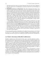
Figure 7.9 illustrates the two-dimensional mesh with five-point stencil (above) and

the sparsity structure of the corresponding coefficient matrix A of Formula (7.17).
In summary, Formulas (7.15) and (7.17) represent a linear equation system with a
sparse coefficient matrix, which has non-zero elements in the main diagonal and its
direct neighbors as well as in the diagonals in distance N . Thus, the linear equation
system resulting from the Poisson equation has a banded structure, which should
be exploited when solving the system. In the following, we present solution meth-
ods for linear equation systems with banded structure and start the description with
tridiagonal systems. These systems have only three non-zero diagonals in the main
diagonal and its two neighbors. A tridiagonal system results, for example, when
discretizing the one-dimensional Poisson equation.
7.2.2 Tridiagonal Systems
For the solution of a linear equation system Ax = y with a banded or tridiagonal
coefficient matrix A ∈ R
n×n
, specific solution methods can exploit the sparse matrix
structure. A matrix A = (a
ij
)
i, j=1, ,n
∈ R
n×n
is called banded when its structure
takes the form of a band of non-zero elements around the principal diagonal. More
precisely, this means a matrix A is a banded matrix if there exists r ∈ N, r ≤ n,
with
a
ij
= 0for|i − j| > r .
The number r is called the semi-bandwidth of A.Forr = 1 a banded matrix
is called tridiagonal matrix. We first consider the solution of tridiagonal systems

which are linear equation systems with tridiagonal coefficient matrix.
7.2.2.1 Gaussian Elimination for Tridiagonal Systems
For the solution of a linear equation system Ax = y with tridiagonal matrix A,
the Gaussian elimination can be used. Step k of the forward elimination (without
pivoting) results in the following computations, see also Sect. 7.1:
1. Compute l
ik
:= a
(k)
ik
/a
(k)
kk
for i = k +1, ,n.
2. Subtract l
ik
times the kth row from the rows i = k +1, ,n, i.e., compute
a
(k+1)
ij
= a
(k)
ij
−l
ik
·a
(k)
kj
for k ≤ j ≤ n and k < i ≤ n .
384 7 Algorithms for Systems of Linear Equations

i-1 i+1i
i-N
i+N
x
23 N1
2N
y
2
N
N+1
(N-1)N+1
12 n
1
2
n
x
x
x
x
x
x
x
x
x
x
x
x
x
x
x

xx
x
xx
x
x
xx
x
x
x
x
xx
x
x
x
x
x
x
x
x
x
N
N
Fig. 7.9 Rectangular mesh in the x–y plane of size N × N and the n × n coefficient matrix
with n = N
2
of the corresponding linear equation system of the five-point formula. The sparsity
structure of the matrix corresponds to the adjacency relation of the mesh points. The mesh can be
considered as adjacency graph of the non-zero elements of the matrix
The vector y is changed analogously.
Because of the tridiagonal structure of A, all matrix elements a

ik
with i ≥ k +2are
zero elements, i.e., a
ik
= 0. Thus, in each step k of the Gaussian elimination only
one elimination factor l
k+1
:= l
k+1,k
and only one row with only one new element
have to be computed. Using the notation
7.2 Direct Methods for Linear Systems with Banded Structure 385
A =
⎛
⎜
⎜
⎜
⎜
⎜
⎜
⎝
b
1
c
1
0
a
2
b
2

c
2
a
3
b
3
.
.
.
.
.
.
.
.
.
c
n−1
0 a
n
b
n
⎞
⎟
⎟
⎟
⎟
⎟
⎟
⎠
(7.20)

for the matrix elements and starting with u
1
= b
1
, these computations are
l
k+1
= a
k+1
/u
k
, (7.21)
u
k+1
= b
k+1
−l
k+1
·c
k
.
After n − 1 steps an LU decomposition A = LU of matrix (7.20) with
L =
⎛
⎜
⎜
⎜
⎝
10
l

2
1
.
.
.
.
.
.
0 l
n
1
⎞
⎟
⎟
⎟
⎠
and U =
⎛
⎜
⎜
⎜
⎝
u
1
c
1
0
.
.
.

.
.
.
u
n−1
c
n−1
0 u
n
⎞
⎟
⎟
⎟
⎠
results. The right-hand side y is transformed correspondingly according to
˜
y
k+1
= y
k+1
−l
k+1
·
˜
y
k
.
The solution x is computed from the upper triangular matrix U by a backward sub-
stitution, starting with x
n

=
˜
y
n
/u
n
and solving the equations u
i
x
i
+c
i
x
i+1
=
˜
y
i
one
after another resulting in
x
i
=
˜
y
i
u
i
−
c

i
u
i
x
i+1
for i = n − 1, ,1 .
The computational complexity of the Gaussian elimination is reduced to O(n)for
tridiagonal systems. However, the elimination phase computing l
k
and u
k
according
to Eq. (7.21) is inherently sequential, since the computation of l
k+1
depends on u
k
and the computation of u
k+1
depends on l
k+1
. Thus, in this form the Gaussian elimi-
nation or LU decomposition has to be computed sequentially and is not suitable for
a parallel implementation.
7.2.2.2 Recursive Doubling for Tridiagonal Systems
An alternative approach for solving a linear equation system with tridiagonal matrix
is the method of recursive doubling or cyclic reduction. The methods of recursive
doubling and cyclic reduction also use elimination steps but contain potential par-
allelism [72, 71]. Both techniques can be applied if the coefficient matrix is either
symmetric and positive definite or diagonal dominant [115]. The elimination steps
386 7 Algorithms for Systems of Linear Equations

in both methods are applied to linear equation systems Ax = y with the matrix
structure shown in (7.20), i.e.,
b
1
x
1
+ c
1
x
2
= y
1
,
a
i
x
i−1
+ b
i
x
i
+ c
i
x
i+1
= y
i
for i = 2, ,n − 1,
a
n

x
n−1
+ b
n
x
n
= y
n
.
The method, which was first introduced by Hockney and Golub in [91], uses two
equations i − 1 and i + 1 to eliminate the variables x
i−1
and x
i+1
from equation
i. This results in a new equivalent equation system with a coefficient matrix with
three non-zero diagonals where the diagonals are moved to the outside. Recursive
doubling and cyclic reduction can be considered as two implementation variants for
the same numerical idea of the method of Hockney and Golub. The implementation
of recursive doubling repeats the elimination step, which finally results in a matrix
structure in which only the elements in the principal diagonal are non-zero and the
solution vector x can be computed easily. Cyclic reduction is a variant of recursive
doubling which also eliminates variables using neighboring rows. But in each step
the elimination is only applied to half of the equations and, thus, less computations
are performed. On the other hand, the computation of the solution vector x requires
a substitution phase.
We would like to mention that the terms recursive doubling and cyclic reduction
are used in different ways in the literature. Cyclic reduction is sometimes used for
the numerical method of Hockney and Golub in both implementation variants, see
[60, 115]. On the other hand the term recursive doubling (or full recursive doubling)

is sometimes used for a different method, the method of Stone [168]. This method
applies the implementation variants sketched above in Eq. (7.21) resulting from
the Gaussian elimination, see [61, 173]. In the following, we start the description of
recursive doubling for the method of Hockney and Golub according to [61] and [13].
Recursive doubling considers three neighboring equations i − 1, i, i + 1of
the equation system Ax = y with coefficient matrix A in the form (7.20) for
i = 3, 4, ,n − 2. These equations are
a
i−1
x
i−2
+ b
i−1
x
i−1
+ c
i−1
x
i
= y
i−1
,
a
i
x
i−1
+ b
i
x
i

+ c
i
x
i+1
= y
i
,
a
i+1
x
i
+ b
i+1
x
i+1
+ c
i+1
x
i+2
= y
i+1
.
Equation i −1isusedtoeliminatex
i−1
from the ith equation and equation i +1is
used to eliminate x
i+1
from the ith equation. This is done by reformulating equations
i − 1 and i +1to
x

i−1
=
y
i−1
b
i−1
−
a
i−1
b
i−1
x
i−2
−
c
i−1
b
i−1
x
i
,
x
i+1
=
y
i+1
b
i+1
−
a

i+1
b
i+1
x
i
−
c
i+1
b
i+1
x
i+2
and inserting those descriptions of x
i−1
and x
i+1
into equation i. The resulting new
equation i is
7.2 Direct Methods for Linear Systems with Banded Structure 387
a
(1)
i
x
i−2
+b
(1)
i
x
i
+c

(1)
i
x
i+2
= y
(1)
i
(7.22)
with coefficients
a
(1)
i
= α
(1)
i
·a
i−1
,
b
(1)
i
= b
i
+α
(1)
i
·c
i−1
+β
(1)

i
·a
i+1
,
c
(1)
i
= β
(1)
i
·c
i+1
, (7.23)
y
(1)
i
= y
i
+α
(1)
i
· y
i−1
+β
(1)
i
· y
i+1
,
and

α
(1)
i
:=−a
i
/b
i−1
,
β
(1)
i
:=−c
i
/b
i+1
.
For the special cases i = 1, 2, n −1, n, the coefficients are given by
b
(1)
1
= b
1
+β
(1)
1
·a
2
, y
(1)
1

= y
1
+β
(1)
1
· y
2
,
b
(1)
n
= b
n
+α
(1)
n
·c
n−1
, y
(1)
n
= b
n
+α
(1)
n
· y
n−1
,
a

(1)
1
= a
(1)
2
= 0, and c
(1)
n−1
= c
(1)
n
= 0 .
The values for a
(1)
n−1
, a
(1)
n
, b
(1)
2
, b
(1)
n−1
, c
(1)
1
, c
(1)
2

, y
(1)
2
, and y
(1)
n−1
are defined as in
Eq. (7.23). Equation (7.22) forms a linear equation system A
(1)
x = y
(1)
with a
coefficient matrix
A
(1)
=
⎛
⎜
⎜
⎜
⎜
⎜
⎜
⎜
⎜
⎜
⎝
b
(1)
1

0 c
(1)
1
0
0 b
(1)
2
0 c
(1)
2
a
(1)
3
0 b
(1)
3
.
.
.
.
.
.
a
(1)
4
.
.
.
.
.

.
.
.
.
c
(1)
n−2
.
.
.
.
.
.
.
.
.
0
0 a
(1)
n
0 b
(1)
n
⎞
⎟
⎟
⎟
⎟
⎟
⎟

⎟
⎟
⎟
⎠
.
Comparing the structure of A
(1)
with the structure of A, it can be seen that the
diagonals are moved to the outside.
In the next step, this method is applied to the equations i − 2, i, i + 2ofthe
equation system A
(1)
x = y
(1)
for i = 5, 6, ,n − 4. Equation i − 2isusedto
eliminate x
i−2
from the ith equation and equation i + 2 is used to eliminate x
i+2
from the ith equation. This results in a new ith equation
a
(2)
i
x
i−4
+b
(2)
i
x
i

+c
(2)
i
x
i+4
= y
(2)
i
,
which contains the variables x
i−4
, x
i
, and x
i+4
. The cases i = 1, ,4, n−3, ,n
are treated separately as shown for the first elimination step. Altogether a next equa-
tion system A
(2)
x = y
(2)
results in which the diagonals are further moved to the
outside. The structure of A
(2)
is
388 7 Algorithms for Systems of Linear Equations
A
(2)
=
⎛

⎜
⎜
⎜
⎜
⎜
⎜
⎜
⎜
⎜
⎜
⎜
⎜
⎜
⎜
⎜
⎜
⎝
b
(2)
1
000c
(2)
1
0
0 b
(2)
2
c
(2)
2

0
.
.
.
.
.
.
0
.
.
.
c
(2)
n−4
a
(2)
5
.
.
.
0
a
(2)
6
.
.
.
0
.
.

.
.
.
.
0
0 a
(2)
n
000b
(2)
n
⎞
⎟
⎟
⎟
⎟
⎟
⎟
⎟
⎟
⎟
⎟
⎟
⎟
⎟
⎟
⎟
⎟
⎠
.

The following steps of the recursive doubling algorithm apply the same method
to the modified equation system of the last step. Step k transfers the side diagonals
2
k
−1 positions away from the main diagonal, compared to the original coefficient
matrix. This is reached by considering equations i − 2
k−1
, i, i +2
k−1
:
a
(k−1)
i−2
k−1
x
i−2
k
+ b
(k−1)
i−2
k−1
x
i−2
k−1
+ c
(k−1)
i−2
k−1
x
i

= y
(k−1)
i−2
k−1
,
a
(k−1)
i
x
i−2
k−1
+ b
(k−1)
i
x
i
+ c
(k−1)
i
x
i+2
k−1
= y
(k−1)
i
,
a
(k−1)
i+2
k−1

x
i
+ b
(k−1)
i+2
k−1
x
i+2
k−1
+ c
(k−1)
i+2
k−1
x
i+2
k
= y
(k−1)
i+2
k−1
.
Equation i − 2
k−1
is used to eliminate x
i−2
k−1
from the ith equation and equation
i +2
k−1
is used to eliminate x

i+2
k−1
from the ith equation. Again, the elimination is
performed by computing the coefficients for the next equation system. These coef-
ficients are
a
(k)
i
= α
(k)
i
·a
(k−1)
i−2
k−1
for i = 2
k
+1, ,n, and a
(k)
i
= 0 otherwise,
c
(k)
i
= β
(k)
i
·c
(k−1)
i+2

k−1
for i = 1, ,n − 2
k
, and c
(k)
i
= 0 otherwise, (7.24)
b
(k)
i
= α
(k)
i
·c
(k−1)
i−2
k−1
+b
(k−1)
i
+β
(k)
i
·a
(k−1)
i+2
k−1
for i = 1, ,n ,
y
(k)

i
= α
(k)
i
· y
(k−1)
i−2
k−1
+ y
(k−1)
i
+β
(k)
i
· y
(k−1)
i+2
k−1
for i = 1, ,n
with
α
(k)
i
:=−a
(k−1)
i
/b
(k−1)
i−2
k−1

for i = 2
k−1
+1, ,n , (7.25)
β
(k)
i
:=−c
(k−1)
i
/b
(k−1)
i+2
k−1
for i = 1, ,n − 2
k−1
.
The modified equation i results by multiplying equation i −2
k−1
from step k −1
with α
(k)
i
, multiplying equation i + 2
k−1
from step k −1 with β
(k)
i
, and adding both
to equation i. The resulting ith equation is
a

(k)
i
x
i−2
k
+b
(k)
i
x
i
+c
(k)
i
x
i+2
k
= y
(k)
i
(7.26)
7.2 Direct Methods for Linear Systems with Banded Structure 389
with the coefficients (7.24). The cases k = 1, 2 are special cases of this formula.
The initialization for k = 0 is the following:
a
(0)
i
= a
i
for i = 2, ,n ,
b

(0)
i
= b
i
for i = 1, ,n ,
c
(0)
i
= c
i
for i = 1, ,n − 1 ,
y
(0)
i
= y
i
for i = 1, ,n .
and a
(0)
1
= 0, c
(0)
n
= 0. Also, for the steps k = 0, ,log n and i ∈ Z \{1, ,n}
the values
a
(k)
i
= c
(k)

i
= y
(k)
i
= 0 ,
b
(k)
i
= 1 ,
x
i
= 0
are set. After N =log nsteps, the original matrix A is transformed into a diagonal
matrix A
(N )
A
(N )
= diag(b
(N )
1
, ,b
(N )
n
)
in which only the main diagonal contains non-zero elements. The solution x of the
linear equation system can be directly computed using this matrix and the corre-
spondingly modified vector y
(N )
:
x

i
= y
(N )
i
/b
(N )
i
for i = 1, 2, ,n .
To summarize, the recursive doubling algorithm consists of two main phases:
1. Elimination phase: Compute the values a
(k)
i
, b
(k)
i
, c
(k)
i
, and y
(k)
i
for k =1, ,log n
and i = 1, ,n according to Eqs. (7.24) and (7.25).
2. Solution phase: Compute x
i
= y
(N )
i
/b
(N )

i
for i = 1, ,n with N =log n.
The first phase consists of log n steps where in each step O(n) values are com-
puted. The sequential asymptotic runtime of the algorithm is therefore O(n ·log n)
which is asymptotically slower than the O(n) runtime for the Gaussian elimination
approach described earlier. The advantage is that the computations in each step of
the elimination and the substitution phase are independent and can be performed in
parallel. Figure 7.10 illustrates the computations of the recursive doubling algorithm
and the data dependencies between different steps.
7.2.2.3 Cyclic Reduction for Tridiagonal Systems
The recursive doubling algorithm offers a large degree of potential parallelism but
has a larger computational complexity than the Gaussian elimination caused by
390 7 Algorithms for Systems of Linear Equations
i=1
i=2
i=3
i=4
i=5
i=6
i=7
i=8
k=0 k=1 k=2 k=3
Fig. 7.10 Dependence graph for the computation steps of the recursive doubling algorithm in the
case of three computation steps and eight equations. The computations of step k are shown in
column k of the illustration. Column k contains one node for each equation i, thus representing the
computation of all coefficients needed in step k. Column 0 represents the data of the coefficient
matrix of the linear system. An edge from a node i in step k to a node j in step k + 1 means that
the computation at node j needs at least one coefficient computed at node i
computational redundancy. The cyclic reduction algorithm is a modification of
recursive doubling which reduces the amount of computations to be performed. In

each step, half the variables in the equation system are eliminated which means that
only half of the values a
(k)
i
, b
(k)
i
, c
(k)
i
, and y
(k)
i
are computed. A substitution phase
is needed to compute the solution vector x. The elimination and the substitution
phases of cyclic reduction are described by the following two phases:
1. Elimination phase: For k = 1, ,log n compute a
(k)
i
, b
(k)
i
, c
(k)
i
, and y
(k)
i
with
i = 2

k
, ,n and step size 2
k
. The number of equations of the form (7.26) is
reduced by a factor of 1/2 in each step. In step k =logn there is only one
equation left for i = 2
N
with N =log n.
2. Substitution phase: For k =log n, ,0 compute x
i
according to Eq. (7.26)
for i = 2
k
, ,n with step size 2
k+1
:
x
i
=
y
(k)
i
−a
(k)
i
· x
i−2
k
−c
(k)

i
· x
i+2
k
b
(k)
i
. (7.27)
Figure 7.11 illustrates the computations of the elimination and the substitution
phases of cyclic reduction represented by nodes and their dependencies represented
by arrows. In each computation step k, k = 1, ,log n, of the elimination phase,
7.2 Direct Methods for Linear Systems with Banded Structure 391
i=1
i=2
i=3
i=4
i=5
i=6
i=7
i=8
k=0 k=1 k=2 k=3
8
x
4
x
x
x
x
x
x

x
2
6
1
3
5
7
Fig. 7.11 Dependence graph illustrating the dependencies between neighboring computation steps
of the cyclic reduction algorithm for the case of three computation steps and eight equations in
analogy to the representation in Fig. 7.10. The first four columns represent the computations of the
coefficients. The last columns in the graph represent the computation of the solution vector x in
the second phase of the cyclic reduction algorithm, see (7.27)
there are n/2
k
nodes representing the computations for the coefficients of one equa-
tion. This results in
n
2
+
n
4
+
n
8
+···+
n
2
N
= n ·
log n


i=1
1
2
i
≤ n
computation nodes with N =log n and, therefore, the execution time of cyclic
reduction is O(n). Thus, the computational complexity is the same as for the
Gaussian elimination; however, the cyclic reduction offers potential parallelism
which can be exploited in a parallel implementation as described in the following.
The computations of the numbers α
(k)
i
, β
(k)
i
require a division by b
(k)
i
and, thus,
cyclic reduction as well as recursive doubling is not possible if any number b
(k)
i
is
zero. This can happen even when the original matrix is invertible and has non-zero
diagonal elements or when the Gaussian elimination can be applied without pivot-
ing. However, for many classes of matrices it can be shown that a division by zero
is never encountered. Examples are matrices A which are symmetric and positive
definite or invertible and diagonally dominant, see [61] or [115] (using the name
odd–even reduction). (A matrix A is symmetric if A = A

T
and positive definite if
x
T
Ax > 0 for all x. A matrix is diagonally dominant if in each row the absolute
value of the diagonal element exceeds the sum of the absolute values of the other
elements in the row without the diagonal in the row.)
392 7 Algorithms for Systems of Linear Equations
7.2.2.4 Parallel Implementation of Cyclic Reduction
We consider a parallel algorithm for the cyclic reduction for p processors. For the
description of the phases we assume n = p ·q for q ∈ N and q = 2
Q
for Q ∈ N.
Each processor stores a block of rows of size q, i.e., processor P
i
stores the rows of
A with the numbers (i − 1)q +1, ,i ·q for 1 ≤ i ≤ p. We describe the parallel
algorithm with data exchange operations that are needed for an implementation with
a distributed address space. As data distribution a row-blockwise distribution of the
matrix A is used to reduce the interaction between processors as much as possible.
The parallel algorithm for the cyclic reduction comprises three phases: the elimina-
tion phase stopping earlier than described above, an additional recursive doubling
phase, and a substitution phase.
Phase 1: Parallel reduction of the cyclic reduction in log q steps: Each pro-
cessor computes the first Q = log q steps of the cyclic reduction algorithm,
i.e., processor P
i
computes for k = 1, ,Q the values
a
(k)

j
, b
(k)
j
, c
(k)
j
, y
(k)
j
for j = (i − 1) ·q + 2
k
, ,i · q with step size 2
k
. After each computation step,
processor P
i
receives four data values from P
i−1
(if i > 1) and from processor P
i+1
(if i < n) computed in the previous step. Since each processor owns a block of
rows of size q, no communication with any other processor is required. The size of
data to be exchanged with the neighboring processors is a multiple of 4 since four
coefficients (a
(k)
j
, b
(k)
j

, c
(k)
j
, y
(k)
j
) are transferred. Only one data block is received per
step and so there are at most 2Q messages of size 4 for each step.
Phase 2: Parallel recursive doubling for tridiagonal systems of size p: Proces-
sor P
i
is responsible for the ith equation of the following p-dimensional tridiagonal
system
˜
a
i
˜
x
i−1
+
˜
b
i
˜
x
i
+
˜
c
i

˜
x
i+1
=
˜
y
i
for i = 1, , p
with
˜
a
i
= a
(Q)
i·q
˜
b
i
= b
(Q)
i·q
˜
c
i
= c
(Q)
i·q
˜
y
i

= y
(Q)
i·q
˜
x
i
= x
i·q
⎫
⎪
⎪
⎪
⎪
⎪
⎪
⎪
⎬
⎪
⎪
⎪
⎪
⎪
⎪
⎪
⎭
for i = 1, ,p .
For the solution of this system, we use recursive doubling. Each processor is
assigned one equation. Processor P
i
performs log p steps of the recursive dou-

bling algorithm. In step k, k = 1, ,log p, processor P
i
computes
˜
a
(k)
i
,
˜
b
(k)
i
,
˜
c
(k)
i
,
˜
y
(k)
i