Engine Testing Theory and Practice P2 ppt
Bạn đang xem bản rút gọn của tài liệu. Xem và tải ngay bản đầy đủ của tài liệu tại đây (311.15 KB, 20 trang )
2 The test cell as a thermodynamic
system
The energy of the world is constant; the entropy strives towards a maximum.
1
Rudolph Clausius (1822–1888)
Introduction
The closed engine test cell system makes a suitable case for students to study an
example of the flow of heat and change in entropy. In almost all engine test cells the
vast majority of the energy comes into the system as highly concentrated ‘chemical
energy’ entering the cell via the smallest penetration in the cell wall, the fuel line.
It leaves the cell as lower grade heat energy via the largest penetrations: the ventilation
duct, engine exhaust pipe and the cooling water pipes. In the case of cells fitted
with electrically regenerative dynamometers, almost one-third of the energy supplied
by fuel will leave the cell as electrical energy able to slow down the electrical
energy supply meter. Many problems are experienced in test cells worldwide when
the thermodynamics of the cell have not been correctly catered for in the design of
cooling systems. The most common problem is high air temperature within the test
cell, either generally or in critical areas. The practical effects of such problems will
be covered in detail in Chapter 5, Ventilation and air conditioning, but it is vital for
the cell designer to have a general appreciation of the contribution of the various
heat sources and the strategies for their control.
In the development of the theory of thermodynamics much use is made of the
concept of the open system. This is a powerful tool and can be very helpful in
considering the total behaviour of a test cell. It is linked to the idea of the control
volume, a space enclosing the system and surrounded by an imaginary surface, the
control surface (Fig. 2.1).
The great advantage of this concept is that once one has identified all the mass
and energy flows into and out of the system it is not necessary to know exactly what
is going on inside the system in order to draw up a ‘balance sheet’ of inflows and
outflows.
The test cell as a thermodynamic system 15
Control surface
Control volume
In
Fuel
Air
Water
Out
Machine
Exhaust
Power
Water
Figure 2.1 An open thermodynamic system
The various inflows and outflows to and from a test cell are as follows:
In
∗
Out
Fuel
Ventilation air (some may be used by
the engine as combustion air)
Ventilation air
Combustion air (treated) Exhaust (includes air used by engine)
Engine cooling water
Charge air (when separately supplied) Dynamometer cooling water
Cooling water Electricity from dynamometer
Electricity for services Losses through walls and ceiling
Balance sheets may be drawn up for fuel, air, water and electricity, but by far
the most important is the energy balance, since every one of these quantities has
associated with it a certain quantity of energy. The same concept may be applied to
the engine within the cell. This may be pictured as surrounded by its own control
surface, through which the following flows take place:
In Out
Fuel Power
Air used by the engine Exhaust
Cooling water Cooling water
Cooling air Cooling air
Convection and radiation
∗
Compressed air may be a further energy input; however, usage is generally intermittent and
unlikely to make a significant contribution.
16 Engine Testing
Measurement of thermal losses from the engine is dealt with in Chapter 13, Thermal
efficiency, measurement of heat and mechanical losses, where the value of the method
in the analysis of engine performance is made clear.
The energy balance of the engine
Table 2.1 shows a possible energy balance sheet for a cell in which a gasoline engine
is developing a steady power output of 100 kW. Note that where fluids (air, water,
exhaust) are concerned, the energy content is referred to an arbitrary zero, the choice
of which is unimportant: we are only interested in the difference between the various
energy flows into and out of the cell.
Given sufficient detailed information on a fixed engine/cell system it is possible
to carry out a very detailed energy balance calculation (see Chapter 5, Ventilation
and air conditioning, for a more detailed treatment). Alternatively there are some
commonly used ‘rule of thumb’ calculations available to the cell designer; the most
common of these relates to the energy balance of the engine which is known as the
‘30–30–30–10 rule’. This refers to the energy balance shown in Table 2.2.
The key lesson to be learnt by the non-specialist reader is that any engine test
cell has to be designed to deal with energy flows that are at least three times greater
than the ‘headline’ engine rating. To many this will sound obvious but a common
fixation on engine power and a casual familiarity with, but lack of appreciation of, the
energy density of petroleum fuels has misled many people in the past to significantly
Table 2.1 Simplified energy flows for a test cell fitted with a hydraulic
dynamometer and 100 kW gasoline engine
Energy balance
In Out
Fuel 300 kW Exhaust gas 60 kW
Ventilating fan power 5 kW Engine cooling water 90 kW
Dynamometer cooling water 95kW
Ventilation air 70 kW
Electricity for cell services 25kW Heat loss, walls and ceiling 15 kW
330 kW 330 kW
The energy balance for the engine, see Chapter 11, is as follows:
In Out
Fuel 300 kW Power 100 kW
Exhaust gas 90 kW
Engine cooling water 90 kW
Convection and radiation 20 kW
300 kW 300 kW
The test cell as a thermodynamic system 17
Table 2.2 Example of the 30–30–30–10 rule
In via Out via
Fuel 300 kW Dynamometer 30% (90 + kW)
Exhaust system 30% (90 kW)
Engine fluids 30% (90 kW)
Convection and radiation 10% (30 kW)
under-rate cell cooling systems. Like any rule of thumb this is crude but does provide
a starting point for the calculation of a full energy balance and a datum from which
we can evaluate significant differences in balance caused by the engine itself and its
mounting within the cell.
Firstly, there are differences inherent in the engine design. Diesels will tend to
transfer less energy into the cell than petrol engines of equal physical size. For
example, testers of rebuilt bus engines often notice that different models of diesels
with the same nominal power output will show quite different distribution of heat
into the test cell air and cooling water.
Secondly, there are differences in engine rigging in the cell which will vary the
temperature and surface area of engine ancillaries, such as exhaust pipes. Finally,
there is the amount and type of equipment within the test cell, all of which makes a
contribution to the convection and radiation heat load to be handled by the ventilation
system.
Specialist designers have developed their own versions of a software model, based
both on empirical data and theoretical calculation, all of which is used within this
book, and which produces the type of energy balance shown in Fig. 2.2. Such tools
are useful but cannot be used uncritically as the final basis of design, particularly
when a range of engines are to be tested or the design has to cover two or more
cells, then the energy diversity factor has to be considered.
Diversity factor and the final specification of a facility
energy balance
To design a multicell test laboratory able to control and dissipate the maximum
theoretical power of all its prime movers on the hottest day of the year will lead to
an oversized system and possibly poor temperature control at low heat outputs. The
amount by which the thermal rating of a facility is reduced from that theoretical maxi-
mum is the diversity factor. In Germany it is called the Gleichzeitigkeits Faktor and is
calculated from zero heat output upwards, rather than 100 per cent heat output down-
wards, but the results should be the same, providing the same assumptions are made.
The diversity factor often lies between 60 and 85 per cent of maximum rating, but
individual systems will vary from endurance beds with high rating down to anechoic
beds with very low rating.
Power output
CFM
CFM
Lights
Fuel
Cooling water to room
0.9%
Process water for
intercooler
Process water for
oil cooling
Process water for
dyno cooling
Combustion air
8.0%
38
Radiation energy
from engine
Ventilation air
Exhaust gas
Exhaust radiation energy
Heat from dyno
cellAC dyno
m
3
/s
12153
91
1.2
28
6.0%
3.2%
15
135
3.8
Electrical power
Electrical service
5
19.5%
12153
5.7
40
919
0.43
150
kW
kW
kW
kW
kW
kW
kW
kW
kW
kW
kW
kW4
kW kW
kW
m
Power output
Instrumentation
m wide
kW
°C
°C
°C
CFM
m
3
/s
CFM
m
3
/s
°C
m
3
/s
°C
kW
kW
kg/kW.h
I/h
469
32.0%
0.262
47.3
0.0%
0.0
33
29.1%
136
55
158
96
5.7
26
499
21
5
6
150
0
0
0.0% 0.0%
4.5%
0.24
25
Energy input
Efficiency
Fuel consumption
Fuel cooling
Total process
water heat load
Process water for
engine cooling
Total heat load
into cell
(
inc. lighting and
building gains
)
Engine
Dyno
Figure 2.2 Output diagram from test cell thermal analysis software
The test cell as a thermodynamic system 19
0
0.2
0.4
0.6
0.8
1
123456
Number of test cells
Diversity factor
Figure 2.3 Diversity factor of thermal rating of facility services, plotted against
number of test cells, based on empirical data from typical automotive test facilities
In calculating, or more correctly estimating, the diversity factor it is essential that
the creators of the operational and functional specifications use realistic values of
actual engine powers, rather than extrapolations based on possible future develop-
ments. A key consideration is the number of cells included within the system. It
is clear that one cell may at some time run at its maximum rating, but it may be
considered less likely that four cells will all run at maximum rating at the same
time: the possible effect of this is shown in Fig. 2.3. There is a degree of bravery
and confidence, based on relevant experience, required to significantly reduce the
theoretical maximum to a contractual specification, but very significant savings in
first and running costs may be possible if it is done correctly.
Once a realistic maximum power rating for the facility has been calculated, the
facility design team can use information concerning the operating regime, planned
test sequences, past records, engine type variation, etc., to draw up diversity factors
for heat energy balance and electrical power requirements. Future proofing may be
better designed into the facility by incremental addition of plant rather than oversizing
at the beginning.
Common or individual services in multicell laboratories?
When considering the thermal loads and the diversity factor of a facility containing
several test cells, it is sensible to consider the strategy to be adopted in the design of
the various services. The choice has to be based on the operation requirements rather
than just the economies of purchasing and running the service modules. Services,
such as cooling water (raw water), are always common and treated via a central
cooling tower system. Services, such as cell ventilation and engine exhaust gas
extraction, may either serve individual cells or are shared. In these cases sharing
may show cost savings and simplify the building design by reducing penetrations;
20 Engine Testing
however, it is prudent to build in some standby or redundancy to prevent total facility
shut-down in the event of, for example, a fan failure.
A problem that must be avoided in the design of common services is ‘cross talk’
between cells where the action in one cell, or other industrial plant, disturbs the
control achieved in another. This is a particular danger when a service, for example
chilled water, has to serve a wide range of thermal loads. In this case a central plant
may be designed to circulate glycol/water mix at 6
C through two or more cells
wherein the coolant is used by devices ranging from large intercoolers to small fuel
conditioners; any sudden increase in demand may significantly increase the system
return temperature and cause an unacceptable disturbance in the control temperatures.
In such systems there needs to be individual control loops per instrument or a
very high thermal inertia gained through the installation of a sufficiently large cold
buffer tank.
Summary
The energy balance approach outlined in this chapter will be found helpful in
analysing the performance of an engine and in the design of test cell services (Chap-
ters 5 and 6). It is recommended that at an early stage in the design of a new test cell,
diagrams such as Fig. 2.2 should be drawn up and labelled with flow and energy
quantities appropriate to the capacity of the engines to be tested.
The large quantities of ventilation air, cooling water, electricity and heat that are
involved will often come as a surprise. Early recognition can help to avoid expensive
wasted design work by ensuring that
•
the general proportions of cell and services do not depart too far from accepted
practice (any large departure is a warning sign);
•
the cell is made large enough to cope with the energy flows involved;
•
sufficient space is allowed for such features as water supply pipes and drains, air
inlet grilles, collecting hoods and exhaust systems. Note that space is not only
required within the test cell but also in any service spaces above or below the
cell and the penetrations within the building envelope.
Reference
1. Eastop, T.D. and McConkey, A. (1993) Applied Thermodynamics for Engineering Tech-
nologists, Longmans, London.
Further reading
Heywood, J.B. (1988) Internal Combustion Engine Fundamentals, McGraw-Hill,
Maidenhead.
3 Vibration and noise
Introduction
Vibration is considered in this chapter with particular reference to the design and oper-
ation of engine test facilities, engine mountings and the isolation of engine-induced
disturbances. Torsional vibration is covered as a separate subject in Chapter 9, Cou-
pling the engine to the dynamometer.
The theory of noise generation and control is briefly considered and a brief account
given of the particular problems involved in the design of anechoic cells.
Vibration and noise
Almost always the engine itself is the only significant source of vibration and noise
in the engine test cell.
1−5
Secondary sources such as the ventilation system, pumps
and circulation systems or the dynamometer are usually swamped by the effects of
the engine.
There are several aspects to this problem:
•
The engine must be mounted in such a way that neither it nor connections to it
can be damaged by excessive movement or excessive constraint.
•
Transmission of engine-induced vibration to the cell structure or to other buildings
must be controlled.
•
Excessive noise levels in the cell should be avoided or contained as far as possible
and the design of alarm signals should take in-cell noise levels into account.
Fundamentals: sources of vibration
Since the vast majority of engines likely to be encountered are single- or multi-
cylinder in-line vertical engines, we shall concentrate on this configuration.
An engine may be regarded as having six degrees of freedom of vibration about
orthogonal axes through its centre of gravity: linear vibrations along each axis and
rotations about each axis (see Fig. 3.1).
22 Engine Testing
Z
Z
X
X
Y
Y
Figure 3.1 Internal combustion engine: principle axes and degrees of freedom
In practice, only three of these modes are usually of importance:
•
vertical oscillations on the X axis due to unbalanced vertical forces;
•
rotation about the Y axis due to cyclic variations in torque;
•
rotation about the Z axis due to unbalanced vertical forces in different transverse
planes.
Torque variations will be considered later. In general, the rotating masses are carefully
balanced but periodic forces due to the reciprocating masses cannot be avoided. The
crank, connecting rod and piston assembly shown in Fig. 3.2 is subject to a periodic
force in the line of action of the piston given approximately by:
f = m
p
2
c
r cos +
m
p
2
c
r cos2
n
where n = l/r (1)
m
f
I
r
ω
c
θ
Figure 3.2 Connecting rod crank mechanism: unbalanced forces
Vibration and noise 23
Here m
p
represents the sum of the mass of the piston plus, by convention, one-third
of the mass of the connecting rod (the remaining two-thirds is usually regarded as
being concentrated at the crankpin centre).
The first term of eq. (1) represents the first-order inertia force. It is equivalent
to the component of centrifugal force on the line of action generated by a mass m
p
concentrated at the crankpin and rotating at engine speed. The second term arises
from the obliquity of the connecting rod and is equivalent to the component of force
in the line of action generated by a mass m/4n at the crankpin radius, but rotating at
twice engine speed.
Inertia forces of higher order (3×,4×, etc., crankshaft speed) are also generated
but may usually be ignored.
It is possible to balance any desired proportion of the first-order inertia force
by balance weights on the crankshaft, but these then give rise to an equivalent
reciprocating force on the Z axis, which may be even more objectionable.
Inertia forces may be represented by vectors rotating at crankshaft speed and twice
crankshaft speed. Table 3.1 shows the first- and second-order vectors for engines
having from one to six cylinders.
Table 3.1 First- and second-order forces, multicylinder engines
First
order
forces
1
1
1
1
1
1
1
1
1
1
1
11
1
1
1
1
1
1
1
1
1
1
1
1
1
1
1
2
2
2
2
2
2
2
2
2
2
2
2
2
2
2
3
3
3
3
3
3
3
5
5
5
5
5
6
6
6
6
5
5
5
3
3
3
3
3
3
3
2
2
2
2
2
3
3
3
3
4
4
4
5
5
6
4
4
4
4
4
4
4
4
4
4
4
4
2
2
2
Second
order
forces
First
order
couples
Second
order
couples
24 Engine Testing
Note the following features:
•
In a single cylinder engine, both first- and second-order forces are unbalanced.
•
For larger numbers of cylinders, first-order forces are balanced.
•
For two and four cylinder engines, the second-order forces are unbalanced and
additive.
This last feature is an undesirable characteristic of a four cylinder engine and in some
cases has been eliminated by counter-rotating weights driven at twice crankshaft
speed.
The other consequence of reciprocating unbalance is the generation of rocking
couples about the transverse or Z axis and these are also shown in Fig. 3.1.
•
There are no couples in a single cylinder engine.
•
In a two cylinder engine, there is a first-order couple.
•
In a three cylinder engine, there are first- and second-order couples.
•
Four and six cylinder engines are fully balanced.
•
In a five cylinder engine, there is a small first-order and a larger second-order
couple.
Six cylinder engines, which are well known for smooth running, are balanced in all
modes.
Variations in engine turning moment are discussed in Chapter 9, coupling the
engine to the dynamometer. These variations give rise to equal and opposite reactions
on the engine, which tend to cause rotation of the whole engine about the crankshaft
axis. The order of these disturbances, i.e. the ratio of the frequency of the disturbance
to the engine speed, is a function of the engine cycle and the number of cylinders.
For a four-stroke engine, the lowest order is equal to half the number of cylinders:
in a single cylinder there is a disturbing couple at half engine speed while in a six
cylinder engine the lowest disturbing frequency is at three times engine speed. In a
two-stroke engine, the lowest order is equal to the number of cylinders.
The design of engine mountings and test bed foundations
The main problem in engine mounting design is that of ensuring that the motions
of the engine and the forces transmitted to the surroundings as a result of the
unavoidable forces and couples briefly described above are kept to manageable
levels. In the case of vehicle engines it is sometimes the practice to make use of the
same flexible mounts and the same location points as in the vehicle; this does not,
however, guarantee a satisfactory solution. In the vehicle, the mountings are carried
on a comparatively light structure, while in the test cell they may be attached to a
massive pallet or even to a seismic block. Also in the test cell the engine may be
fitted with additional equipment and various service connections. All of these factors
alter the dynamics of the system when compared with the situation of the engine in
Vibration and noise 25
service and can give rise to fatigue failures of both the engine support brackets and
those of auxiliary devices, such as the alternator.
Truck diesel engines usually present less of a problem than small automotive
engines, as they generally have fairly massive and well-spaced supports at the fly-
wheel end. Stationary engines will in most cases be carried on four or more flexible
mountings in a single plane below the engine and the design of a suitable system is
a comparatively simple matter.
We shall consider the simplest case, an engine of mass m kg carried on undamped
mountings of combined stiffness k N/m (Fig. 3.3). The differential equation defining
the motion of the mass equates the force exerted by the mounting springs with the
acceleration of the mass:
md
2
x
dt
2
+ kx = 0(2)
a solution is
x = cons tant × sin
k
m
· t
k
m
=
2
0
natural frequency =
0
=
0
2
=
1
2
k
m
(3)
the static deflection under the force of gravity = mg/k which leads to a very convenient
expression for the natural frequency of vibration:
0
=
1
2
g
static deflection
(4a)
C of G
Figure 3.3 Engine carried on four flexible mountings
26 Engine Testing
or, if static deflection is in millimetres:
0
=
1576
√
static deflection
(4b)
This relationship is plotted in Fig. 3.4
Next, consider the case where the mass m is subjected to an exciting force of
amplitude f and frequency /2. The equation of motion now reads:
m
d
2
x
dt
2
+kx =f sint
the solution includes a transient element; for the steady state condition amplitude of
oscillation is given by:
x =
f/k
1−
2
/
2
0
(5)
here f/k is the static deflection of the mountings under an applied load f. This
expression is plotted in Fig. 3.5 in terms of the amplitude ratio x divided by static
deflection. It has the well-known feature that the amplitude becomes theoretically
infinite at resonance, =
0
.
If the mountings combine springs with an element of viscous damping, the equa-
tion of motion becomes:
m
d
2
x
dt
2
+c
dx
dt
+kx =f sint
40
30
20
10
5
4
3
2
1
0.2
Natural frequency (Hz)
0.5 1 2 5
Static deflection (mm)
10 20 50 100 300
Figure 3.4 Relationship between static deflection and natural frequency
Vibration and noise 27
6
4
2
0
0
Amplitude ratio
12
Frequency ratio
ω
0
ω
Figure 3.5 Relationship between frequency and amplitude ratio (transmissibil-
ity) undamped vibration
where c is a damping coefficient. The steady state solution is:
x =
f/k
1−
2
2
0
2
+
2
c
2
mk
2
0
sint −A (6a)
If we define a dimensionless damping ratio:
C
2
=
c
2
4mk
this equation may be written:
x =
f/k
1−
2
2
0
2
+4C
2
2
2
0
sint −A (6b)
(if C =1 we have the condition of critical damping when, if the mass is displaced
and released, it will return eventually to its original position without overshoot).
The amplitude of the oscillation is given by the first part of this expression:
amplitude =
f/k
1−
2
2
0
2
+4C
2
2
2
0
28 Engine Testing
10
0
0.05
0.1
0.1
0
0.2
0.2
0.5
0.5
0.05
5
2
1
0.8
0.6
0.4
0.3
0.2
0.1
0.08
0.06
0.04
0.03
0.02
0
0.1 0.2
Transmissibility
0.5 1 2 3 4 5 7 10
Frequency ratio
ω
0
ω
C
Figure 3.6 Relationship between transmissibility (amplitude ratio) and fre-
quency, damped oscillations for different values of damping ratio C (logarithmic
plot)
This is plotted in Fig. 3.6, together with the curve for the undamped condition,
Fig. 3.5, and various values of C are shown. The phase angle A is a measure of the
angle by which the motion of the mass lags or leads the exciting force. It is given
by the expression:
A =tan
−1
2C
0
0
−
0
(7)
At very low frequencies, A is zero and the mass moves in phase with the exciting force.
With increasing frequency the motion of the mass lags by an increasing angle, reach-
ing 90
at resonance. At high frequencies the sign of A changes and the mass leads
the exciting force by an increasing angle, approaching 180
at high ratios of to
0
.
Natural rubber flexible mountings have an element of internal (hysteresis) damping
which corresponds approximately to a degree of viscous damping corresponding to
C =0.05.
Vibration and noise 29
The essential role of damping will be clear from Fig. 3.6: it limits the potentially
damaging amplitude of vibration at resonance. The ordinate in Fig. 3.6 is often
described as the transmissibility of the mounting system: it is a measure of the extent
to which the disturbing force f is reduced by the action of the flexible mounts. It is
considered good practice to design the system so that the minimum speed at which
the machine is to run is not less than three times the natural frequency, corresponding
to a transmissibility of about 0.15. It should be noticed that once the frequency
ratio exceeds about 2 the presence of damping actually has an adverse effect on the
isolation of disturbing forces.
Practical considerations in the design of engine and test bed
mountings
In the above simple treatment we have only considered oscillations in the vertical
direction. In practice, as has already been pointed out, an engine carried on flexible
mountings has six degrees of freedom (Fig. 3.1). While in many cases a simple
analysis of vibrations in the vertical direction will give a satisfactory result, under test
cell conditions a more complete computer analysis of the various modes of vibration
and the coupling between them may be advisable. This is particularly the case with
tall engines with mounting points at a low level, when cyclic variations in torque
may induce transverse rolling of the engine.
Reference 6 lists the design factors to be considered in planning a system for the
isolation and control of vibration and transmitted noise:
•
specification of force isolation
– as attenuation, dB
– as transmissibility
– as efficiency
– as noise level in adjacent rooms
•
natural frequency range to achieve the level of isolation required
•
load distribution of the machine
– is it equal on each mounting?
– is the centre of gravity low enough for stability?
– exposure to forces arising from connecting services, exhaust system, etc.
•
vibration amplitudes – low frequency
– normal operation
– fault conditions
– starting and stopping
– is a seismic block or sub-base needed?
30 Engine Testing
•
higher-frequency structure-borne noise (100 Hz+)
– is there a specification?
– details of building structure
– sufficient data on engine and associated plant
•
transient forces
– shocks, earthquakes, machine failures
•
environment
– temperature
– humidity
– fuel and oil spills.
Detailed design of engine mountings for test bed installation is a highly specialized
matter, see Ker-Wilson
1
for guidance on standard practice. In general, the aim is to
avoid ‘coupled’ vibrations, e.g. the generation of pitching forces due to unbalanced
forces in the vertical direction, or the generation of rolling moments due to the torque
reaction forces exerted by the engine. These can give rise to resonances at much
higher frequencies than the simple frequency of vertical oscillation calculated in the
following section and to consequent trouble, particularly with the engine-to-brake
connecting shaft.
Massive foundations and supported bedplates
The analysis and prediction of the extent of transmitted vibration to the surroundings
is a highly specialized field. The theory is dealt with in Ref. 1, the starting point being
the observation that a heavy block embedded in the earth has a natural frequency
of vibration that generally lies within the range 1000 to 2000c.p.m. There is thus
a possibility of vibration being transmitted to the surroundings if exciting forces,
generally associated with the reciprocating masses in the engine, lie within this
frequency range. An example would be a four cylinder four-stroke engine running
at 750 rev/min. We see from Table 3.1 that such an engine generates substantial
second-order forces at twice engine speed or 1500c.p.m. Figure 3.7, redrawn from
Ref. 1, gives an indication of acceptable levels of transmitted vibration from the
point of view of physical comfort.
Figure 3.8 is a sketch of a typical seismic block. Reinforced concrete weighs
roughly 2500 kg/m
3
and this block would weigh about 4500 kg. Note that the sur-
rounding tread plates must be isolated from the block, also that it is essential to
electrically earth (ground) the mounting rails. The block is shown carried on four
combined steel spring and rubber isolators, each having a stiffness of 100 kg/mm
(Fig. 3.9). From eq. 2a, the natural frequency of vertical oscillation of the bare
block would be 4.70 Hz or 282 c.p.m., so the block would be a suitable base for an
engine running at about 900 rev/min or faster. If the engine weight were, say, 500 kg
Vibration and noise 31
7
2
1
0.7
0.2
0.1
0.07
0.02
0.01
0.007
0.002
100 200 500
Rough
Normal
Smooth
Perceptible
Imperceptible
Frequency c.p.m.
Amplitude mm
1000 2000 5000
Figure 3.7 Perception of vibration
+
–
12 m
0.8 m
Figure 3.8 Spring-mounted seismic block
32 Engine Testing
Resilient pads
Resilient pad
Assembly bolt and snubber
Slot to inspect
snubber position
Base casting
Top casting
Rubber spring
Helical steel spring
Figure 3.9 Combined spring and rubber flexible mount
the natural frequency of block and engine would be reduced to 4.46Hz, a negligible
change. An ideal design target for the natural frequency is considered to be 3 Hz.
Heavy concrete foundations (seismic blocks) carried on a flexible membrane are
expensive to construct, calling for deep excavations, complex shuttering and elaborate
arrangements, such as tee-slotted bases, for bolting down the engines. With the wide
range of different types of flexible mounting now available, it is questionable whether,
except in special circumstances, such as a requirement to install test facilities in close
proximity to offices, their use is economically justified. The trough surrounding the
block may be of incidental use for installing services, if the gap is small then there
should be means of draining out contaminated fluid spills.
It is now common practice for automotive engines to be rigged on vehicle type
engine mounts, then on trolley systems, which are themselves mounted on isolation
feet therefore less engine vibration is transmitted to the building floor. In these
cases a more modern alternative to the deep seismic block is shown in Fig. 3.10a
and is sometimes used where the soil conditions are suitable. Here the test bed
sits on a thickened and isolated section of the floor cast in situ on the compacted
native ground. The gap between the floor and block is almost filled with expanded
polystyrene boards and sealed at floor level with a flexible, fuel resistant, sealant. A
damp-proof membrane should be inserted under both floor and pit or block.
Where the subsoil is not suitable for the arrangement shown in Fig. 3.10a then
a pit is required, cast to support a concrete block that sits on a mat or pads of a
material such as cork/nitrile rubber composite which is resistant to fluid contamination
(Fig. 3.10b), alternatively a cast iron bedplate supported by air springs, as shown in
Figure 3.11, may be installed.
Vibration and noise 33
(a)
Consolidated subsoil
Cell floor
Seismic block
Isolation gap filled with fuel resistant
sealant
Cell floor
Seismic block
placed on
resilient mat
Concrete pit
(b)
Figure 3.10 (a) Isolated foundation block for test stand set on to firm subsoil;
(b) seismic block on to resilient matting in a shallow pit
4
2
1
5
3
Figure 3.11 Seismic block or cast bedplate (not shown) (4) mounted on air
springs (3) within a shallow concrete pit (2) on consolidated subsoil (1). When
the air supply is off the self-levelling air springs allow the block to settle on
support blocks (5) the rise and fall typically being 4 to 6 mm. Maintenance
access to the springs is not shown