statistical and adaptive signal processing

Statistical
and Adaptive
Signal Processing

Recent Titles in the Artech House Signal Processing Library
Computer Speech Technology, Robert D. Rodman
Digital Signal Processing and Statistical Classification, George J. Miao and
Mark A. Clements
Handbook of Neural Networks for Speech Processing,
Shigeru Katagiri, editor
Hilbert Transforms in Signal Processing, Stefan L. Hahn
Phase and Phase-Difference Modulation in Digital Communications,
Yuri Okunev
Signal Processing Fundamentals and Applications for Communications and Sensing
Systems, John Minkoff
Signals, Oscillations, and Waves: A Modern Approach, David Vakman
Statistical Signal Characterization, Herbert L. Hirsch
Statistical Signal Characterization Algorithms and Analysis Programs, Herbert L. Hirsch
Voice Recognition, Richard L. Klevans and Robert D. Rodman
For further information on these and other Artech House titles, including previously
considered out-of-print books now available through our In-Print-Forever
®
(IPF
®
)
program, contact:
Artech House Artech House
685 Canton Street 46 Gillingham Street
Norwood, MA 02062 London SW1V 1AH UK
Phone: 781-769-9750 Phone: +44 (0)20 7596-8750

Fax: 781-769-6334 Fax: +44 (0)20 7630-0166
e-mail: e-mail:
Find us on the World Wide Web at: www.artechhouse.com

Statistical
and Adaptive
Signal Processing
Spectral Estimation, Signal Modeling, Adaptive
Filtering, and Array Processing
Dimitris G. Manolakis
Massachusetts Institute of Technology
Lincoln Laboratory
Vinay K. Ingle
Northeastern University
Stephen M. Kogon
Massachusetts Institute of Technology
Lincoln Laboratory
a
r
tec
hh
ouse
.
co
m
Library of Congress Cataloging-in-Publication Data
A catalog record for this book is available from the U.S. Library of Congress.
British Library Cataloguing in Publication Data
A catalogue record for this book is available from the British Library.
This is a reissue of a McGraw-Hill book.

Cover design by Igor Valdman
© 2005 ARTECH HOUSE, INC.
685 Canton Street
Norwood, MA 02062
All rights reserved. Printed and bound in the United States of America. No part of this
book may be reproduced or utilized in any form or by any means, electronic or
mechanical, including photocopying, recording, or by any information storage and
retrieval system, without permission in writing from the publisher.
All terms mentioned in this book that are known to be trademarks or service marks
have been appropriately capitalized. Artech House cannot attest to the accuracy of this
information. Use of a term in this book should not be regarded as affecting the validity of
any trademark or service mark.
International Standard Book Number: 1-58053-610-7
10 9 8 7 6 5 4 3 2 1
To my beloved wife, Anna, and to the loving memory of my father, Gregory.
DGM
To my beloved wife, Usha, and adoring daughters, Natasha and Trupti.
VKI
To my wife and best friend, Lorna, and my children, Gabrielle and Matthias.
SMK
ABOUT THE AUTHORS
DIMITRIS G. MANOLAKIS, a native of Greece, received his education (B.S. in physics
and Ph.D. in electrical engineering) from the University of Athens, Greece. He is currently
a member of the technical staff at MIT Lincoln Laboratory, in Lexington, Massachusetts.
Previously, he was a Principal Member, Research Staff, at Riverside Research Institute. Dr.
Manolakis has taught at the University of Athens, Northeastern University, Boston College,
and Worcester Polytechnic Institute; and he is coauthor of the textbook Digital Signal
Processing: Principles, Algorithms, and Applications (Prentice-Hall, 1996, 3d ed.). His
research experience and interests include the areas of digital signal processing, adaptive
filtering, array processing, pattern recognition, and radar systems.

VINAY K. INGLE is Associate Professor of Electrical and Computer Engineering at
Northeastern University. He received his Ph.D. in eletrical and computer engineering from
Rensselaer Polytechnic Institute in 1981. He has broad research experience and has taught
courses on topics including signal and image processing, stochastic processes, and
estimation theory. Professor Ingle is coauthor of the textbooks DSP Laboratory Using the
ADSP-2101 Microprocessor (Prentice-Hall, 1991) and DSP Using Matlab (PWS
Publishing Co., Boston, 1996).
STEPHEN M. KOGON received the Ph.D. degree in electrical engineering from Georgia
Institute of Technology. He is currently a member of the technical staff at MIT Lincoln
Laboratory in Lexington, Massachusetts. Previously, he has been associated with Raytheon
Co., Boston College, and Georgia Tech Research Institute. His research interests are in the
areas of adaptive processing, array signal processing, radar, and statisticalsignalmodeling.
CONTENTS
Preface xvii
1 Introduction 1
1.1 Random Signals 1
1.2 Spectral Estimation 8
1.3 Signal Modeling 11
1.3.1 Rational or Pole-Zero
Models / 1.3.2 Fractional
Pole-Zero Models and
Fractal Models
1.4 Adaptive Filtering 16
1.4.1 Applications of Adaptive
Filters / 1.4.2 Features of
Adaptive Filters
1.5 Array Processing 25
1.5.1 Spatial Filtering or
Beamforming / 1.5.2 Adaptive
Interference Mitigation in

Radar Systems / 1.5.3 Adaptive
Sidelobe Canceler
1.6 Organization of the Book 29
2 Fundamentals of Discrete-
Time Signal Processing
33
2.1 Discrete-Time Signals 33
2.1.1 Continuous-Time, Discrete-
Time, and Digital Signals /
2.1.2 Mathematical Description of
Signals / 2.1.3 Real-World Signals
2.2 Transform-Domain
Representation of
Deterministic Signals
37
2.2.1 Fourier Transforms and
Fourier Series / 2.2.2 Sampling
of Continuous-Time Signals /
2.2.3 The Discrete Fourier
Transform / 2.2.4 The
z-Transform / 2.2.5 Representation
of Narrowband Signals
2.3 Discrete-Time Systems 47
2.3.1 Analysis of Linear,
Time-Invariant Systems / 2.3.2
Response to Periodic Inputs / 2.3.3
Correlation Analysis and Spectral
Density
2.4 Minimum-Phase and
System Invertibility 54

2.4.1 System Invertibility and
Minimum-Phase Systems /
2.4.2 All-Pass Systems / 2.4.3
Minimum-Phase and All-Pass
Decomposition / 2.4.4 Spectral
Factorization
2.5 Lattice Filter Realizations 64
2.5.1 All-Zero Lattice Structures /
2.5.2 All-Pole Lattice Structures
2.6 Summary 70
Problems 70
3 Random Variables, Vectors,
and Sequences
75
3.1 Random Variables 75
3.1.1 Distribution and Density
Functions / 3.1.2 Statistical
Averages / 3.1.3 Some Useful
Random Variables
3.2 Random Vectors 83
3.2.1 Definitions and Second-Order
Moments / 3.2.2 Linear
Transformations of Random
Vectors / 3.2.3 Normal Random
Vectors / 3.2.4 Sums of Independent
Random Variables
3.3 Discrete-Time Stochastic
Processes 97
3.3.1 Description Using
Probability Functions / 3.3.2

Second-Order Statistical
Description / 3.3.3 Stationarity /
x
e56toc.qxd 3/16/05 11:56 AM Page x
xi
Contents
3.3.4 Ergodicity / 3.3.5 Random
Signal Variability / 3.3.6
Frequency-Domain Description
of Stationary Processes
3.4 Linear Systems with
Stationary Random Inputs 115
3.4.1 Time-Domain Analysis /
3.4.2 Frequency-Domain Analysis /
3.4.3 Random Signal Memory /
3.4.4 General Correlation
Matrices / 3.4.5 Correlation
Matrices from Random Processes
3.5 Whitening and Innovations
Representation
125
3.5.1 Transformations Using
Eigen-decomposition / 3.5.2
Transformations Using
Triangular Decomposition /
3.5.3 The Discrete Karhunen-
Loève Transform
3.6 Principles of Estimation
Theory
133

3.6.1 Properties of Estimators /
3.6.2 Estimation of Mean /
3.6.3 Estimation of Variance
3.7 Summary 142
Problems
143
4 Linear Signal Models
149
4.1 Introduction 149
4.1.1 Linear Nonparametric
Signal Models / 4.1.2 Parametric
Pole-Zero Signal Models / 4.1.3
Mixed Processes and the Wold
Decomposition
4.2 All-Pole Models 156
4.2.1 Model Properties /
4.2.2 All-Pole Modeling and
Linear Prediction / 4.2.3
Autoregressive Models
/ 4.2.4
Lower-Order Models
4.3 All-Zero Models 172
4.3.1 Model Properties / 4.3.2
Moving-Average Models / 4.3.3
Lower-Order Models
4.4 Pole-Zero Models 177
4.4.1 Model Properties / 4.4.2
Autoregressive Moving-Average
Models / 4.4.3 The First-Order
Pole-Zero Model 1: PZ (1, 1) /

4.4.4 Summary and Dualities
4.5 Models with Poles
on the Unit Circle 182
4.6 Cepstrum of Pole-Zero
Models 184
4.6.1 Pole-Zero Models / 4.6.2
All-Pole Models / 4.6.3 All-Zero
Models
4.7 Summary 189
Problems 189
5 Nonparametric Power
Spectrum Estimation
195
5.1 Spectral Analysis of
Deterministic Signals 196
5.1.1 Effect of Signal Sampling /
5.1.2 Windowing, Periodic
Extension, and Extrapolation /
5.1.3 Effect of Spectrum
Sampling / 5.1.4 Effects of
Windowing: Leakage and Loss
of Resolution / 5.1.5 Summary
5.2 Estimation of the
Autocorrelation of
Stationary Random Signals 209
5.3 Estimation of the Power
Spectrum of Stationary
Random Signals 212
5.3.1 Power Spectrum Estimation
Using the Periodogram / 5.3.2

Power Spectrum Estimation by
Smoothing a Single Periodogram—
The Blackman-Tukey Method /
5.3.3 Power Spectrum Estimation
by Averaging Multiple
Periodograms—The Welch-
Bartlett Method / 5.3.4 Some
Practical Considerations and
Examples
e56toc.qxd 3/16/05 11:56 AM Page xi
xii
Contents
5.4 Joint Signal Analysis 237
5.4.1 Estimation of Cross-Power
Spectrum / 5.4.2 Estimation of
Frequency Response Functions
5.5 Multitaper Power
Spectrum Estimation 246
5.5.1 Estimation of Auto Power
Spectrum / 5.5.2 Estimation
of Cross Power Spectrum
5.6 Summary 254
Problems 255
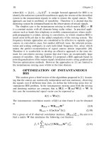
6 Optimum Linear Filters
261
6.1 Optimum Signal
Estimation 261
6.2 Linear Mean Square
Error Estimation 264
6.2.1 Error Performance Surface /

6.2.2 Derivation of the Linear
MMSE Estimator / 6.2.3 Principal-
Component Analysis of the Optimum
Linear Estimator / 6.2.4 Geometric
Interpretations and the Principle of
Orthogonality / 6.2.5 Summary
and Further Properties
6.3 Solution of the Normal
Equations 274
6.4 Optimum Finite Impulse
Response Filters 278
6.4.1 Design and Properties /
6.4.2 Optimum FIR Filters for
Stationary Processes / 6.4.3
Frequency-Domain Interpretations
6.5 Linear Prediction 286
6.5.1 Linear Signal Estimation /
6.5.2 Forward Linear Prediction /
6.5.3 Backward Linear Prediction /
6.5.4 Stationary Processes /
6.5.5 Properties
6.6 Optimum Infinite Impulse
Response Filters 295
6.6.1 Noncausal IIR Filters /
6.6.2 Causal IIR Filters / 6.6.3
Filtering of Additive Noise / 6.6.4
Linear Prediction Using the
Infinite Past—Whitening
6.7 Inverse Filtering
and Deconvolution 306

6.8 Channel Equalization in Data
Transmission Systems 310
6.8.1 Nyquist’s Criterion for Zero
ISI / 6.8.2 Equivalent Discrete-Time
Channel Model / 6.8.3 Linear
Equalizers / 6.8.4 Zero-Forcing
Equalizers / 6.8.5 Minimum MSE
Equalizers
6.9 Matched Filters and
Eigenfilters 319
6.9.1 Deterministic Signal in Noise /
6.9.2 Random Signal in Noise
6.10 Summary 325
Problems 325
7 Algorithms and Structures
for Optimum Linear Filters
333
7.1 Fundamentals of Order-
Recursive Algorithms 334
7.1.1 Matrix Partitioning and
Optimum Nesting / 7.1.2 Inversion
of Partitioned Hermitian Matrices /
7.1.3 Levinson Recursion for the
Optimum Estimator / 7.1.4 Order-
Recursive Computation of the LDL
H
Decomposition / 7.1.5 Order-
Recursive Computation of the
Optimum Estimate
7.2 Interpretations of

Algorithmic Quantities 343
7.2.1 Innovations and Backward
Prediction / 7.2.2 Partial
Correlation / 7.2.3 Order
Decomposition of the Optimum
Estimate / 7.2.4 Gram-Schmidt
Orthogonalization
7.3 Order-Recursive Algorithms
for Optimum FIR Filters 347
7.3.1 Order-Recursive Computation
of the Optimum Filter / 7.3.2
e56toc.qxd 3/16/05 11:56 AM Page xii
xiii
Contents
Lattice-Ladder Structure / 7.3.3
Simplifications for Stationary
Stochastic Processes / 7.3.4
Algorithms Based on the UDU
H
Decomposition
7.4 Algorithms of Levinson
and Levinson-Durbin 355
7.5 Lattice Structures for
Optimum FIR Filters
and Predictors 361
7.5.1 Lattice-Ladder Structures /
7.5.2 Some Properties and
Interpretations / 7.5.3 Parameter
Conversions
7.6 Algorithm of Schür 368

7.6.1 Direct Schür Algorithm /
7.6.2 Implementation
Considerations / 7.6.3 Inverse
Schür Algorithm
7.7 Triangularization and Inversion
of Toeplitz Matrices 374
7.7.1 LDL
H
Decomposition of
Inverse of a Toeplitz Matrix /
7.7.2 LDL
H
Decomposition of a
Toeplitz Matrix / 7.7.3 Inversion
of Real Toeplitz Matrices
7.8 Kalman Filter Algorithm
378
7.8.1 Preliminary Development /
7.8.2 Development of Kalman Filter
7.9 Summary 387
Problems
389
8 Least-Squares Filtering
and Prediction
395
8.1 The Principle of Least
Squares 395
8.2 Linear Least-Squares
Error Estimation 396
8.2.1 Derivation of the Normal

Equations / 8.2.2 Statistical
Properties of Least-Squares
Estimators
8.3 Least-Squares FIR Filters 406
8.4 Linear Least-Squares
Signal Estimation 411
8.4.1 Signal Estimation and Linear
Prediction / 8.4.2 Combined
Forward and Backward Linear
Prediction (FBLP) / 8.4.3
Narrowband Interference
Cancelation
8.5 LS Computations Using the
Normal Equations 416
8.5.1 Linear LSE Estimation /
8.5.2 LSE FIR Filtering and
Prediction
8.6 LS Computations Using
Orthogonalization
Techniques 422
8.6.1 Householder Reflections /
8.6.2 The Givens Rotations / 8.6.3
Gram-Schmidt Orthogonalization
8.7 LS Computations Using
the Singular Value
Decomposition 431
8.7.1 Singular Value
Decomposition / 8.7.2 Solution
of the LS Problem / 8.7.3
Rank-Deficient LS Problems

8.8 Summary 438
Problems 439
9 Signal Modeling
and Parametric
Spectral Estimation
445
9.1 The Modeling Process:
Theory and Practice 445
9.2 Estimation of All-Pole
Models
449
9.2.1 Direct Structures /
9.2.2 Lattice Structures / 9.2.3
Maximum Entropy Method / 9.2.4
Excitations with Line Spectra
9.3 Estimation of Pole-Zero
Models 462
9.3.1 Known Excitation / 9.3.2
Unknown Excitation / 9.3.3
e56toc.qxd 3/16/05 11:56 AM Page xiii
xiv
Contents
Nonlinear Least-Squares
Optimization
9.4 Applicatons 467
9.4.1 Spectral Estimation /
9.4.2 Speech Modeling
9.5 Minimum-Variance
Spectrum Estimation 471
9.6 Harmonic Models and

Frequency Estimation
Techniques
478
9.6.1 Harmonic Model /
9.6.2 Pisarenko Harmonic
Decomposition / 9.6.3 MUSIC
Algorithm / 9.6.4 Minimum-Norm
Method / 9.6.5 ESPRIT Algorithm
9.7 Summary 493
Problems 494
10 Adaptive Filters
499
10.1 Typical Applications of
Adaptive Filters
500
10.1.1 Echo Cancelation in
Communications / 10.1.2
Equalization of Data
Communications Channels /
10.1.3 Linear Predictive Coding /
10.1.4 Noise Cancelation
10.2 Principles of
Adaptive Filters 506
10.2.1 Features of Adaptive
Filters / 10.2.2 Optimum versus
Adaptive Filters / 10.2.3 Stability
and Steady-State Performance of
Adaptive Filters / 10.2.4 Some
Practical Considerations
10.3 Method of

Steepest Descent 516
10.4 Least-Mean-Square
Adaptive Filters 524
10.4.1 Derivation / 10.4.2
Adaptation in a Stationary SOE /
10.4.3 Summary and Design
Guidelines / 10.4.4 Applications
of the LMS Algorithm / 10.4.5
Some Practical Considerations
10.5 Recursive Least-Squares
Adaptive Filters 548
10.5.1 LS Adaptive Filters /
10.5.2 Conventional Recursive
Least-Squares Algorithm / 10.5.3
Some Practical Considerations /
10.5.4 Convergence and
Performance Analysis
10.6 RLS Algorithms
for Array Processing 560
10.6.1 LS Computations Using
the Cholesky and QR
Decompositions / 10.6.2 Two
Useful Lemmas / 10.6.3 The
QR-RLS Algorithm /
10.6.4 Extended QR-RLS
Algorithm / 10.6.5 The Inverse
QR
-RLS Algorithm / 10.6.6
Implementation of QR-RLS
Algorithm Using the Givens

Rotations / 10.6.7 Implementation
of Inverse QR-RLS Algorithm
Using the Givens Rotations /
10.6.8 Classification of RLS
Algorithms for Array Processing
10.7 Fast RLS Algorithms
for FIR Filtering 573
10.7.1 Fast Fixed-Order RLS FIR
Filters / 10.7.2 RLS Lattice-
Ladder Filters / 10.7.3 RLS
Lattice-Ladder Filters Using Error
Feedback Updatings / 10.7.4
Givens Rotation–Based LS Lattice-
Ladder Algorithms / 10.7.5
Classification of RLS Algorithms
for FIR Filtering
10.8 Tracking Performance
of Adaptive Algorithms 590
10.8.1 Approaches for
Nonstationary SOE / 10.8.2
Preliminaries in Performance
Analysis / 10.8.3 The LMS
Algorithm / 10.8.4 The RLS
Algorithm with Exponential
Forgetting / 10.8.5 Comparison
of Tracking Performance
10.9 Summary
607
Problems 608
e56toc.qxd 3/16/05 11:56 AM Page xiv

xv
Contents
11 Array Processing 621
11.1 Array Fundamentals 622
11.1.1 Spatial Signals / 11.1.2
Modulation-Demodulation /
11.1.3 Array Signal Model /
11.1.4 The Sensor Array: Spatial
Sampling
11.2 Conventional Spatial
Filtering: Beamforming
631
11.2.1 Spatial Matched Filter /
11.2.2 Tapered Beamforming
11.3 Optimum Array
Processing 641
11.3.1 Optimum Beamforming /
11.3.2 Eigenanalysis of the
Optimum Beamformer / 11.3.3
Interference Cancelation
Performance / 11.3.4 Tapered
Optimum Beamforming / 11.3.5
The Generalized Sidelobe Canceler
11.4 Performance
Considerations for
Optimum Beamformers 652
11.4.1 Effect of Signal Mismatch /
11.4.2 Effect of Bandwidth
11.5 Adaptive Beamforming
659

11.5.1 Sample Matrix Inversion /
11.5.2 Diagonal Loading with the
SMI Beamformer / 11.5.3
Implementation of the SMI
Beamformer / 11.5.4 Sample-by-
Sample Adaptive Methods
11.6 Other Adaptive Array
Processing Methods 671
11.6.1 Linearly Constrained
Minimum-Variance Beamformers /
11.6.2 Partially Adaptive Arrays /
11.6.3 Sidelobe Cancelers
1 1.7 Angle Estimation 678
11.7.1 Maximum-Likelihood
Angle Estimation / 11.7.2
Cramér-Rao Lower Bound on
Angle Accuracy / 11.7.3
Beamsplitting Algorithms /
11.7.4 Model-Based Methods
11.8 Space-Time
Adaptive Processing 683
11.9 Summary 685
Problems 686
12 Further Topics 691
12.1 Higher-Order Statistics
in Signal Processing 691
12.1.1 Moments, Cumulants, and
Polyspectra / 12.1.2 Higher-
Order Moments and LTI Systems /
12.1.3 Higher-Order Moments of

Linear Signal Models
12.2 Blind Deconvolution
697
12.3 Unsupervised Adaptive
Filters—Blind Equalizers 702
12.3.1 Blind Equalization /
12.3.2 Symbol Rate Blind
Equalizers / 12.3.3 Constant-
Modulus Algorithm
12.4 Fractionally Spaced
Equalizers
709
12.4.1 Zero-Forcing Fractionally
Spaced Equalizers / 12.4.2
MMSE Fractionally Spaced
Equalizers / 12.4.3 Blind
Fractionally Spaced Equalizers
12.5 Fractional Pole-Zero
Signal Models 716
12.5.1 Fractional Unit-Pole
Model / 12.5.2 Fractional Pole-
Zero Models: FPZ (p, d, q) /
12.5.3 Symmetric a-Stable
Fractional Pole-Zero Processes
12.6 Self-Similar Random
Signal Models 725
12.6.1 Self-Similar Stochastic
Processes / 12.6.2 Fractional
Brownian Motion / 12.6.3
Fractional Gaussian Noise /

12.6.4 Simulation of Fractional
Brownian Motions and Fractional
Gaussian Noises / 12.6.5
Estimation of Long Memory /
e56toc.qxd 3/16/05 11:56 AM Page xv
xvi
Contents
12.6.6 Fractional Lévy Stable
Motion
12.7 Summary 741
Problems 742
Appendix A Matrix Inversion
Lemma
745
Appendix B Gradients and
Optimization in
Complex Space
747
B.1 Gradient 747
B.2 Lagrange Multipliers
749
Appendix C MATLAB
Functions 753
Appendix D Useful Results
from Matrix Algebra
755
D.1 Complex-Valued
Vector Space 755
Some Definitions
D.2 Matrices 756

D.2.1 Some Definitions / D.2.2
Properties of Square Matrices
D.3 Determinant of a Square
Matrix 760
D.3.1 Properties of the
Determinant / D.3.2 Condition
Number
D.4 Unitary Matrices 762
D.4.1 Hermitian Forms after
Unitary Transformations / D.4.2
Significant Integral of Quadratic
and Hermitian Forms
D.5 Positive Definite Matrices 764
Appendix E Minimum Phase
Test for Polynomials
767
Bibliography 769
Index 787
e56toc.qxd 3/16/05 11:56 AM Page xvi
March 9, 2005 14:24 e56-pre Sheet number 1 Page number xvii black
xvii
One must learn by doing the thing;
for though you think you know it
You have no certainty, until you try.
—Sophocles, Trachiniae
PREFACE
The principal goal of this book is to provide a unified introduction to the theory, imple-
mentation, and applications of statistical and adaptive signal processing methods. We have
focused on the key topics of spectral estimation, signal modeling, adaptive filtering, and ar-
ray processing, whose selection was based on the grounds of theoretical value and practical

importance. The book has been primarily written with students and instructors in mind. The
principal objectives are to provide an introduction to basic concepts and methodologies that
can provide the foundation for further study, research, and application to new problems.
To achieve these goals, we have focused on topics that we consider fundamental and have
either multiple or important applications.
APPROACH AND PREREQUISITES
The adopted approach is intended to help both students and practicing engineers understand
the fundamental mathematical principles underlying the operation of a method, appreciate
its inherent limitations, and provide sufficient details for its practical implementation. The
academic flavor of this book has been influenced by our teaching whereas its practical
character has been shaped by our research and development activities in both academia and
industry. The mathematical treatment throughout this book has been kept at a level that is
within the grasp of upper-level undergraduate students, graduate students, and practicing
electrical engineers with a background in digital signal processing, probability theory, and
linear algebra.
ORGANIZATION OF THE BOOK
Chapter 1 introduces the basic concepts and applications of statistical and adaptive signal
processing and provides an overview of the book. Chapters 2 and 3 review the fundamentals
of discrete-time signal processing, study random vectors and sequences in the time and
frequency domains, and introduce some basic concepts of estimation theory. Chapter 4
provides a treatment of parametric linear signal models (both deterministic and stochastic)
in the time and frequency domains. Chapter 5 presents the most practical methods for
the estimation of correlation and spectral densities. Chapter 6 provides a detailed study
of the theoretical properties of optimum filters, assuming that the relevant signals can be
modeled as stochastic processes with known statistical properties; and Chapter 7 contains
algorithms and structures for optimum filtering, signal modeling, and prediction. Chapter
March 9, 2005 14:24 e56-pre Sheet number 2 Page number xviii black
xviii
Preface
8 introduces the principle of least-squares estimation and its application to the design of

practical filters and predictors. Chapters 9, 10, and 11 use the theoretical work in Chapters
4, 6, and 7 and the practical methods in Chapter 8, to develop, evaluate, and apply practical
techniques for signal modeling, adaptive filtering, and array processing. Finally, Chapter 12
introduces some advanced topics: definition and properties of higher-order moments, blind
deconvolution and equalization, and stochastic fractional and fractal signal models with long
memory. Appendix A contains a review of the matrix inversion lemma,Appendix B reviews
optimization in complex space, Appendix C contains a list of the Matlab functions used
throughout the book, Appendix D provides a review of useful results from matrix algebra,
and Appendix E includes a proof for the minimum-phase condition for polynomials.
THEORY AND PRACTICE
It is our belief that sound theoretical understanding goes hand-in-hand with practical im-
plementation and application to real-world problems. Therefore, the book includes a large
number of computer experiments that illustrate important concepts and help the reader
to easily implement the various methods. Every chapter includes examples, problems,
and computer experiments that facilitate the comprehension of the material. To help the
reader understand the theoretical basis and limitations of the various methods and apply
them to real-world problems, we provide Matlab functions for all major algorithms and
examples illustrating their use. The Matlab files and additional material about the book can
be found at />manolakismatlab.html. A Solutions Manual with detailed solutions to all the prob-
lems is available to the instructors adopting the book for classroom use.
Dimitris G. Manolakis
Vinay K. Ingle
Stephen M. Kogon
February 2, 2005 11:00 e56-ch1 Sheet number 1 Page number 1 black
1
CHAPTER 1
Introduction
This book is an introduction to the theory and algorithms used for the analysis and pro-
cessing of random signals and their applications to real-world problems. The fundamental
characteristic of random signals is captured in the following statement: Although random

signals are evolving in time in an unpredictable manner, their average statistical proper-
ties exhibit considerable regularity. This provides the ground for the description of random
signals using statistical averages instead of explicit equations. When we deal with random
signals, the main objectives are the statistical description, modeling, and exploitation of the
dependence between the values of one or more discrete-time signals and their application
to theoretical and practical problems.
Random signals are described mathematically by using the theory of probability, ran-
dom variables, and stochastic processes. However, in practice we deal with random signals
by using statistical techniques. Within this framework we can develop, at least in princi-
ple, theoretically optimum signal processing methods that can inspire the development and
can serve to evaluate the performance of practical statistical signal processing techniques.
The area of adaptive signal processing involves the use of optimum and statistical signal
processing techniques to design signal processing systems that can modify their charac-
teristics, during normal operation (usually in real time), to achieve a clearly predefined
application-dependent objective.
The purpose of this chapter is twofold: to illustrate the nature of random signals with
some typical examples and to introduce the four major application areas treated in this book:
spectral estimation, signal modeling, adaptive filtering, and array processing. Throughout
the book, the emphasis is on the application of techniques to actual problems in which the
theoretical framework provides a foundation to motivate the selection of a specific method.
1.1 RANDOM SIGNALS
A discrete-time signal or time series is a set of observations taken sequentially in time,
space, or some other independent variable. Examples occur in various areas, including
engineering, natural sciences, economics, social sciences, and medicine.
A discrete-time signal x(n) is basically a sequence of real or complex numbers called
samples. Although the integer index n may represent any physical variable (e.g., time,
distance), we shall generally refer to it as time. Furthermore, in this book we consider only
time series with observations occurring at equally spaced intervals of time.
Discrete-time signals can arise in several ways. Very often, a discrete-time signal is
obtained by periodically sampling a continuous-time signal, that is, x(n) = x

c
(nT ), where
T = 1/F
s
(seconds) is the sampling period and F
s
(samples per second or hertz) is the
sampling frequency. At other times, the samples of a discrete-time signal are obtained
February 2, 2005 11:00 e56-ch1 Sheet number 2 Page number 2 black
2
chapter 1
Introduction
by accumulating some quantity (which does not have an instantaneous value) over equal
intervals of time, for example, the number of cars per day traveling on a certain road.
Finally, some signals are inherently discrete-time, for example, daily stock market prices.
Throughout the book, except if otherwise stated, the terms signal, time series, or sequence
will be used to refer to a discrete-time signal.
The key characteristics of a time series are that the observations are ordered in time and
that adjacent observations are dependent (related). To see graphically the relation between
the samples of a signal that are l sampling intervals away, we plot the points {x(n), x(n +l)}
for 0 ≤ n ≤ N − 1 − l, where N is the length of the data record. The resulting graph is
known as the l lag scatter plot. This is illustrated in Figure 1.1, which shows a speech signal
and two scatter plots that demonstrate the correlation between successive samples. We note
that for adjacent samples the data points fall close to a straight line with a positive slope.
This implies high correlation because every sample is followed by a sample with about the
same amplitude. In contrast, samples that are 20 sampling intervals apart are much less
correlated because the points in the scatter plot are randomly spread.
When successiveobservations of theseries aredependent, we mayuse past observations
to predict future values. If the prediction is exact, the series is said to be deterministic.
However, in most practical situations we cannot predict a time series exactly. Such time

500 1000 1500 2000 2500 3000 3500
−0.3
−0.2
−0.1
0
0.1
0.2
0.3
Sample number
Amplitude
Signal
−0.4 −0.2 0 0.2 0.4
−0.3
−0.2
−0.1
0
0.1
0.2
0.3
x(n)
x(n–1)
−0.4
−0.2 0 0.2 0.4
−0.3
−0.2
−0.1
0
0.1
0.2
0.3

x(n)
x(n−20)
(a)
(b)
FIGURE 1.1
(a) The waveform for the speech signal “signal”;(b) two scatter plots for successive samples and samples
separated by 20 sampling intervals.
February 2, 2005 11:00 e56-ch1 Sheet number 3 Page number 3 black
3
section 1.1
Random Signals
series are called random or stochastic, and the degree of their predictability is determined
by the dependence between consecutive observations. The ultimate case of randomness
occurs when every sample of a random signal is independent of all other samples. Such a
signal, which is completely unpredictable, is known as white noise and is used as a building
block to simulate random signals with different types of dependence. To summarize, the
fundamental characteristic of a random signal is the inability to precisely specify its values.
In other words, a random signal is not predictable, it never repeats itself, and we cannot find
a mathematical formula that provides its values as a function of time. As a result, random
signals can only be mathematically described by using the theory of stochastic processes
(see Chapter 3).
This book provides an introduction to the fundamental theory and a broad selection
of algorithms widely used for the processing of discrete-time random signals. Signal pro-
cessing techniques, dependent on their main objective, can be classified as follows (see
Figure 1.2):
•
Signal analysis. The primary goal is to extract useful information that can be used to
understand the signal generation process or extract features that can be used for signal
classification purposes. Most of the methods in this area are treated under the disciplines
of spectral estimation and signal modeling. Typical applications include detection and

classification of radar and sonar targets, speech and speaker recognition, detection and
classification of natural and artificial seismic events, event detection and classification in
biological and financial signals, efficient signal representation for data compression, etc.
•
Signal filtering. The main objective ofsignal filtering is to improve the quality of a signal
according to an acceptable criterion of performance. Signal filtering can be subdivided
into the areas of frequency selective filtering, adaptive filtering, and array processing.
Typical applications include noiseandinterferencecancelation,echocancelation, channel
equalization, seismic deconvolution, active noise control, etc.
We conclude this section with some examples of signals occurring in practical applications.
Although the desciption of these signals is far from complete, we provide sufficient infor-
mation to illustrate their random nature and significance in signal processing applications.
Random signals
Analysis
Theory of stochastic
processes,
estimation, and
optimum filtering
Filtering
Spectral
estimation
Signal modeling
(Chapters 4, 8,
Adaptive filtering
12)
Array processing
(Chapters 5, 9)
9, 12)
(Chapters 8, 10,
(Chapter 11)

(Chapters 2, 3, 6, 7)
FIGURE 1.2
Classification of methods for the analysis and processing of random signals.
February 2, 2005 11:00 e56-ch1 Sheet number 4 Page number 4 black
4
chapter 1
Introduction
Speech signals. Figure 1.3 shows the spectrogram and speech waveform correspond-
ing to the utterance “signal.” The spectrogram is a visual representation of the distribution
of the signal energy as a function of time and frequency. We note that the speech signal has
significant changes in both amplitude level and spectral content across time. The waveform
contains segments of voiced (quasi-periodic) sounds, such as “e,” and unvoiced or fricative
(noiselike) sounds, such as “g.”
0 0.05 0.1 0.15 0.2 0.25 0.3 0.35 0.4
−0.2
0
0.2
Time (s)
Amplitude
Signal
Time (s)
Frequency (Hz)
0 0.05 0.1 0.15 0.2 0.25 0.3 0.35 0.4
0
1000
2000
3000
4000
FIGURE 1.3
Spectrogram and acoustic waveform for the utterance “signal.” The horizontal dark bands show the resonances of the

vocal tract, which change as a function of time depending on the sound or phoneme being produced.
Speech production involves three processes: generation of the sound excitation, artic-
ulation by the vocal tract, and radiation from the lips and/or nostrils. If the excitation is
a quasi-periodic train of air pressure pulses, produced by the vibration of the vocal cords,
the result is a voiced sound. Unvoiced sounds are produced by first creating a constriction
in the vocal tract, usually toward the mouth end. Then we generate turbulence by forc-
ing air through the constriction at a sufficiently high velocity. The resulting excitation is a
broadband noiselike waveform.
The spectrum of the excitation is shaped by the vocal tract tube, which has a frequency
response that resembles the resonances of organ pipes or wind instruments. The resonant
frequencies of the vocal tract tube are known as formant frequencies, or simply formants.
Changing the shape of the vocal tract changes its frequency response and results in the
generation of different sounds. Since the shape of the vocal tract changes slowly during
continuous speech, we usually assume that it remains almost constant over intervals on the
order of 10 ms. More details about speech signal generation and processing can be found
in Rabiner and Schafer 1978; O’Shaughnessy 1987; and Rabiner and Juang 1993.
Electrophysiological signals. Electrophysiologywasestablishedinthe late eighteenth
centurywhenGalvanidemonstratedthepresenceofelectricityinanimaltissues.Today,elec-
trophysiological signals play a prominent role in every branch of physiology, medicine, and
February 2, 2005 11:00 e56-ch1 Sheet number 5 Page number 5 black
5
section 1.1
Random Signals
biology. Figure1.4 shows a setof typical signals recorded in a sleep laboratory (Rechtschaf-
fen and Kales 1968). The most prominent among them is the electroencephalogram (EEG),
whose spectral content changes to reflect the state of alertness and the mental activity of
the subject. The EEG signal exhibits some distinctive waves, known as rhythms, whose
dominant spectral content occupies certain bands as follows: delta (δ), 0.5 to 4 Hz; theta
(θ), 4 to 8 Hz; alpha (α), 8 to 13 Hz; beta (β), 13 to 22 Hz; and gamma (γ ), 22 to 30 Hz.
During sleep, if the subject is dreaming, the EEG signal shows rapid low-amplitude fluctu-

ations similar to those obtained in alert subjects, and this is known as rapid eye movement
(REM) sleep. Some other interesting features occurring during nondreaming sleep periods
resemble alphalike activity and are known as sleep spindles. More details can be found in
Duffy et al. 1989 and Niedermeyer and Lopes Da Silva 1998.
FIGURE 1.4
Typical sleep laboratory recordings. The two top signals show eye movements, the next one
illustrates EMG (electromyogram) or muscle tonus, and the last one illustrates brain waves
(EEG) during the onset of a REM sleep period (from Rechtschaffen and Kales 1968).
The beat-to-beat fluctuations in heart rate and other cardiovascular variables, suchasar-
terial blood pressure and stroke volume, are mediated by the joint activityofthesympathetic
and parasympathetic systems. Figure 1.5 shows time series for the heart rate and systolic ar-
terial blood pressure. We note that both heart rate and blood pressure fluctuate in a complex
manner that depends on the mental or physiological state of the subject. The individual or
joint analysis of such time series can help to understand the operation of the cardiovascular
system, predict cardiovascular diseases, and help in the development of drugs and devices
for cardiac-related problems (Grossman et al. 1996; Malik and Camm 1995; Saul 1990).
Geophysical signals. Remote sensing systems use a variety of electro-optical sensors
that span the infrared, visible, and ultraviolet regions of the spectrum and find many civilian
and defense applications. Figure 1.6 shows two segments of infrared scans obtained by a
space-based radiometer looking down at earth (Manolakis et al. 1994). The shape of the
profiles depends on the transmission properties of the atmosphere and the objects in the
radiometer’s field-of-view (terrain or sky background). The statistical characterization and
modeling of infrared backgrounds are critical for the design of systems to detect missiles
against such backgrounds as earth’s limb, auroras, and deep-space star fields (Sabins 1987;
Colwell1983).Othergeophysicalsignalsof interest are recordings ofnaturalandman-made
seismiceventsandseismicsignals usedingeophysicalprospecting(Bolt 1993;Dobrin1988;
Sheriff 1994).
February 2, 2005 11:00 e56-ch1 Sheet number 6 Page number 6 black
6
chapter 1

Introduction
0 100 200 300 400 500 600
50
55
60
65
70
75
Beats/minute
Heart rate
0 100 200 300 400 500 600
150
160
170
180
190
200
Systolic blood pressure
Time (s)
FIGURE 1.5
Simultaneous recordings of the heart rate and systolic blood pressure signals for a
subject at rest.
0 200 400 600 800 1000 1200 1400
49.0
49.5
50.0
50.5
51.0
51.5
52.0

Radiance
Infrared 1
0 200 400 600 800 1000 1200 1400
35
40
45
50
Sample index
Radiance
Infrared 2
FIGURE 1.6
Time series of infrared radiation measurements obtained by a scanning radiometer.
February 2, 2005 11:00 e56-ch1 Sheet number 7 Page number 7 black
7
section 1.1
Random Signals
Radar signals. We conveniently define a radar system to consist of both a transmitter
and a receiver. When the transmitter and receiver are colocated, the radar system is said to
be monostatic, whereas if they are spatially separated, the system is bistatic. The radar first
transmits a waveform, which propagates through space as electromagnetic energy, and then
measures the energy returned to the radar via reflections. When the returns are due to an
object of interest, the signal is known as a target, while undesired reflectionsfromtheearth’s
surface are referred to as clutter. In addition, the radar may encounter energy transmitted by
a hostile opponent attempting to jam the radar and prevent detection of certain targets. Col-
lectively, clutter and jamming signals are referred to as interference. The challenge facing
the radar system is how to extract the targets of interest in the presence of sometimes severe
interference environments. Target detection is accomplished by using adaptive processing
methods that exploit characteristics of the interference in order to suppress these undesired
signals.
A transmitted radar signal propagates through space as electromagnetic energy at ap-

proximately the speed of light c = 3 × 10
8
m/s. The signal travels until it encounters an
object that reflects the signal’s energy. A portion of the reflected energy returns to the radar
receiver along the same path. The round-trip delay of the reflected signal determines the
distance or range of the object from the radar. The radar has a certain receive aperture,
either a continuous aperture or one made up of a series of sensors. The relative delay of a
signal as it propagates across the radar aperture determines its angle of arrival, or bearing.
The extent of the aperture determines the accuracy to which the radar can determine the
direction of a target. Typically, the radar transmits a series of pulses at a rate known as the
pulse repetition frequency. Any target motion produces a phase shift in the returns from
successive pulses caused by the Doppler effect. This phase shift across the series of pulses
is known as the Doppler frequency of the target, which in turn determines the target radial
velocity. The collection of these various parameters (range, angle, and velocity) allows the
radar to locate and track a target.
An example of a radar signal as a function of range in kilometers (km) is shown in
Figure 1.7. The signal is made up of a target, clutter, and thermal noise.All the signals have
been normalized with respect to the thermal noise floor. Therefore, the normalized noise
has unit variance (0 dB). The target signal is at a range of 100 km with a signal-to-noise
ratio (SNR) of 15 dB. The clutter, on the other hand, is present at all ranges and is highly
nonstationary. Its power levels vary from approximately 40 dB at near ranges down to the
thermal noise floor (0 dB) at far ranges. Part of the nonstationarity in the clutter is due to
the range falloff of the clutter as its power is attenuated as a function of range. However, the
rises and dips present between 100 and 200 km are due to terrain-specific artifacts. Clearly,
the target is not visible, and the clutter interference must be removed or canceled in order
50 100 150 200 250
−20
0
20
40

60
Range (km)
Power-to-noise-ratio (dB)
FIGURE 1.7
Example of a radar return signal, plotted as relative power with
respect to noise versus range.