Recursive macroeconomic theory, Thomas Sargent 2nd Ed - Chapter 2 pptx

Chapter 2
Time series
2.1. Two workhorses
This chapter describes two tractable models of time series: Markov chains and
first-order stochastic linear difference equations. These models are organizing
devices that put particular restrictions on a sequence of random vectors. They
are useful because they describe a time series with parsimony. In later chapters,
we shall make two uses each of Markov chains and stochastic linear difference
equations: (1) to represent the exogenous information flows impinging on an
agent or an economy, and (2) to represent an optimum or equilibrium outcome
of agents’ decision making. The Markov chain and the first-order stochastic
linear difference both use a sharp notion of a state vector. A state vector sum-
marizes the information about the current position of a system that is relevant
for determining its future. The Markov chain and the stochastic linear difference
equation will be useful tools for studying dynamic optimization problems.
2.2. Markov chains
A stochastic process is a sequence of random vectors. For us, the sequence will
be ordered by a time index, taken to be the integers in this book. So we study
discrete time models. We study a discrete state stochastic process with the
following property:
Markov Property: A stochastic process {x
t
} is said to have the Markov
property if for all k ≥ 1andallt,
Prob (x
t+1
|x
t
,x
t−1
, ,x

t−k
)=Prob(x
t+1
|x
t
) .
We assume the Markov property and characterize the process by a Markov
chain. A time-invariant Markov chain is defined by a triple of objects, namely,
– 26 –
Markov chains 27
an n-dimensional state space consisting of vectors e
i
,i =1, ,n,wheree
i
is
an n × 1 unit vector whose ith entry is 1 and all other entries are zero; an
n ×n transition matrix P , which records the probabilities of moving from one
value of the state to another in one period; and an (n ×1) vector π
0
whose ith
element is the probability of being in state i at time 0: π
0i
=Prob(x
0
= e
i
).
The elements of matrix P are
P
ij

=Prob(x
t+1
= e
j
|x
t
= e
i
) .
For these interpretations to be valid, the matrix P and the vector π must satisfy
the following assumption:
Assumption M:
a. For i =1, ,n,thematrixP satisfies
n

j=1
P
ij
=1. (2.2.1)
b. The vector π
0
satisfies
n

i=1
π
0i
=1.
AmatrixP that satisfies property (2.2.1) is called a stochastic matrix.A
stochastic matrix defines the probabilities of moving from each value of the state

to any other in one period. The probability of moving from one value of the
state to any other in two periodsisdeterminedbyP
2
because
Prob (x
t+2
= e
j
|x
t
= e
i
)
=
n

h=1
Prob (x
t+2
= e
j
|x
t+1
= e
h
)Prob(x
t+1
= e
h
|x

t
= e
i
)
=
n

h=1
P
ih
P
hj
= P
(2)
ij
,
where P
(2)
ij
is the i, j element of P
2
.LetP
(k)
i,j
denote the i, j element of P
k
.
By iterating on the preceding equation, we discover that
Prob (x
t+k

= e
j
|x
t
= e
i
)=P
(k)
ij
.
28 Time series
The unconditional probability distributions of x
t
are determined by
π

1
=Prob(x
1
)=π

0
P
π

2
=Prob(x
2
)=π


0
P
2
.
.
.
π

k
=Prob(x
k
)=π

0
P
k
,
where π

t
=Prob(x
t
)isthe(1×n) vector whose ith element is Prob(x
t
= e
i
).
2.2.1. Stationary distributions
Unconditional probability distributions evolve according to
π


t+1
= π

t
P. (2.2.2)
An unconditional distribution is called stationary or invariant if it satisfies
π
t+1
= π
t
,
that is, if the unconditional distribution remains unaltered with the passage of
time. From the law of motion (2.2.2) for unconditional distributions, a station-
ary distribution must satisfy
π

= π

P (2.2.3)
or
π

(I −P )=0.
Transposing both sides of this equation gives
(I − P

) π =0, (2.2.4)
which determines π as an eigenvector (normalized to satisfy


n
i=1
π
i
=1)
associated with a unit eigenvalue of P

.
The fact that P is a stochastic matrix (i.e., it has nonnegative elements
and satisfies

j
P
ij
=1foralli) guarantees that P has at least one unit
eigenvalue, and that there is at least one eigenvector π that satisfies equation
(2.2.4). This stationary distribution may not be unique because P can have a
repeated unit eigenvalue.
Markov chains 29
Example 1.AMarkovchain
P =


100
.2 .5 .3
001


has two unit eigenvalues with associated stationary distributions π


=[1 0 0]
and π

= [ 0 0 1 ]. Here states 1 and 3 are both absorbing states. Further-
more, any initial distribution that puts zero probability on state 2 is a stationary
distribution. See exercises 1.10 and 1.11.
Example 2.AMarkovchain
P =


.7 .30
0 .5 .5
0 .9 .1


has one unit eigenvalue with associated stationary distribution π

=[0 .6429 .3571].
Herestates2and3formanabsorbing subset of the state space.
2.2.2. Asymptotic stationarity
We often ask the following question about a Markov process: for an arbitrary
initial distribution π
0
, do the unconditional distributions π
t
approach a sta-
tionary distribution
lim
t→∞
π

t
= π
∞
,
where π
∞
solves equation (2.2.4)? If the answer is yes, then does the limit
distribution π
∞
depend on the initial distribution π
0
? If the limit π
∞
is inde-
pendent of the initial distribution π
0
, we say that the process is asymptotically
stationary with a unique invariant distribution. We call a solution π
∞
a sta-
tionary distribution or an invariant distribution of P .
We state these concepts formally in the following definition:
Definition: Let π
∞
be a unique vector that satisfies (I −P

)π
∞
=0. If for
all initial distributions π

0
it is true that P
t
π
0
converges to the same π
∞
,we
say that the Markov chain is asymptotically stationary with a unique invariant
distribution.
The following theorems can be used to show that a Markov chain is asymp-
totically stationary.
30 Time series
Theorem 1: Let P be a stochastic matrix with P
ij
> 0 ∀(i, j). Then P has
a unique stationary distribution, and the process is asymptotically stationary.
Theorem 2: Let P be a stochastic matrix for which P
n
ij
> 0 ∀(i, j)forsome
value of n ≥ 1. Then P has a unique stationary distribution, and the process
is asymptotically stationary.
The conditions of theorem 1 (and 2) state that from any state there is a positive
probability of moving to any other state in 1 (or n)steps.
2.2.3. Expectations
Let y be an n×1 vector of real numbers and define y
t
= y


x
t
,sothaty
t
= y
i
if
x
t
= e
i
. From the conditional and unconditional probability distributions that
we have listed, it follows that the unconditional expectations of y
t
for t ≥ 0are
determined by Ey
t
=(π

0
P
t
)y . Conditional expectations are determined by
E (y
t+1
|x
t
= e
i
)=


j
P
ij
y
j
=(Py)
i
(2.2.5)
E (y
t+2
|x
t
= e
i
)=

k
P
(2)
ik
y
k
=

P
2
y

i

(2.2.6)
and so on, where P
(2)
ik
denotes the (i, k)elementofP
2
.Noticethat
E [E (y
t+2
|x
t+1
= e
j
) |x
t
= e
i
]=

j
P
ij

k
P
jk
y
k
=


k



j
P
ij
P
jk


y
k
=

k
P
(2)
ik
y
k
= E (y
t+2
|x
t
= e
i
) .
Connecting the first and last terms in this string of equalities yields E[E(y
t+2

|x
t+1
)|x
t
]=
E[y
t+2
|x
t
]. This is an example of the ‘law of iterated expectations’. The law of
iterated expectations states that for any random variable z and two information
sets J, I with J ⊂ I , E[E(z|I)|J]=E(z|J). As another example of the law of
iterated expectations, notice that
Ey
1
=

j
π
1,j
y
j
= π

1
y =(π

0
P ) y = π


0
(P y)
Markov chains 31
and that
E [E (y
1
|x
0
= e
i
)] =

i
π
0,i

j
P
ij
y
j
=

j


i
π
0,i
P

ij

y
j
= π

1
y = Ey
1
.
2.2.4. Forecasting functions
There are powerful formulas for forecasting functions of a Markov process. Again
let
y be an n ×1 vector and consider the random variable y
t
= y

x
t
.Then
E [y
t+k
|x
t
= e
i
]=

P
k

y

i
where (P
k
y)
i
denotes the ith row of P
k
y . Stacking all n rows together, we
express this as
E [y
t+k
|x
t
]=P
k
y. (2.2.7)
We also have
∞

k=0
β
k
E [y
t+k
|x
t
= e
i

]=

(I − βP)
−1
y

i
,
where β ∈ (0, 1) guarantees existence of (I − βP)
−1
=(I + βP + β
2
P
2
+ ···).
One-step-ahead forecasts of a sufficiently rich set of random variables char-
acterize a Markov chain. In particular, one-step-ahead conditional expectations
of n independent functions (i.e., n linearly independent vectors h
1
, ,h
n
)
uniquely determine the transition matrix P .Thus,letE[h
k,t+1
|x
t
= e
i
]=
(Ph

k
)
i
. We can collect the conditional expectations of h
k
for all initial states
i in an n × 1 vector E[h
k,t+1
|x
t
]=Ph
k
. We can then collect conditional ex-
pectations for the n independent vectors h
1
, ,h
n
as Ph = J where h =
[ h
1
h
2
h
n
]andJ is an the n×n matrix of all conditional expectations
of all n vectors h
1
, ,h
n
.Ifweknowh and J ,wecandetermineP from

P = Jh
−1
.
32 Time series
2.2.5. Invariant functions and ergodicity
Let P, π be a stationary n-state Markov chain with the same state space we
have chosen above, namely, X =[e
i
,i =1, ,n]. An n × 1 vector y defines
a random variable y
t
= y

x
t
. Thus, a random variable is another term for
‘function of the underlying Markov state’.
The following is a useful precursor to a law of large numbers:
Theorem 2.2.1. Let
y define a random variable as a function of an underlying
state x,wherex is governed by a stationary Markov chain (P, π).Then
1
T
T

t=1
y
t
→ E [y
∞

|x
0
](2.2.8)
with probability 1.
Here E[y
∞
|x
0
] is the expectation of y
s
for s very large, conditional on
the initial state. We want more than this. In particular, we would like to
be able to replace E[y
∞
|x
0
] with the constant unconditional mean E[y
t
]=
E[y
0
] associated with the stationary distribution. To get this requires that we
strengthen what is assumed about P by using the following concepts. First, we
use
Definition 2.2.1. A random variable y
t
= y

x
t

is said to be invariant if
y
t
= y
0
,t≥ 0, for any realization of x
t
,t≥ 0.
Thus, a random variable y is invariant (or ‘an invariant function of the state’)
if it remains constant while the underlying state x
t
moves through the state
space X .
For a finite state Markov chain, the following theorem gives a convenient
way to characterize invariant functions of the state.
Theorem 2.2.2. Let P, π be a stationary Markov chain. If
E [y
t+1
|x
t
]=y
t
(2.2.9)
then the random variable y
t
= y

x
t
is invariant.

Markov chains 33
Proof. By using the law of iterated expectations, notice that
E (y
t+1
− y
t
)
2
= E

E

y
2
t+1
− 2y
t+1
y
t
+ y
2
t

|x
t

= E

Ey
2

t+1
|x
t
− 2E (y
t+1
|x
t
) y
t
+ Ey
2
t
|x
t

= Ey
2
t+1
− 2Ey
2
t
+ Ey
2
t
=0
where the middle term in the right side of the second line uses that E[y
t
|x
t
]=y

t
,
the middle term on the right side of the third line uses the hypothesis (2.2.9),
and the third line uses the hypothesis that π is a stationary distribution. In a
finite Markov chain, if E(y
t+1
− y
t
)
2
=0,then y
t+1
= y
t
for all y
t+1
,y
t
that
occur with positive probability under the stationary distribution.
As we shall have reason to study in chapters 16 and 17, any (non necessarily
stationary) stochastic process y
t
that satisfies (2.2.9) is said to be a martingale.
Theorem 2.2.2 tells us that a martingale that is a function of a finite state
stationary Markov state x
t
must be constant over time. This result is a special
case of the martingale convergence theorem that underlies some remarkable
results about savings to be studied in chapter 16.

1
Equation (2.2.9)canbeexpressedasP y = y or
(P − I)
y =0, (2.2.10)
which states that an invariant function of the state is a (right) eigenvector of P
associated with a unit eigenvalue.
Definition 2.2.2. Let (P, π) be a stationary Markov chain. The chain is said
to be ergodic if the only invariant functions
y are constant with probability one,
i.e.,
y
i
= y
j
for all i, j with π
i
> 0,π
j
> 0.
A law of large numbers for Markov chains is:
Theorem 2.2.3. Let
y define a random variable on a stationary and ergodic
Markov chain (P, π).Then
1
T
T

t=1
y
t

→ E [y
0
](2.2.11)
1
Theorem 2.2.2 tells us that a stationary martingale process has so little
freedom to move that it has to be constant forever, not just eventually as asserted
by the martingale convergence theorem.
34 Time series
with probability 1.
This theorem tells us that the time series average converges to the popula-
tion mean of the stationary distribution.
Three examples illustrate these concepts.
Example 1. A chain with transition matrix P =

01
10

has a unique invariant
distribution π =[.5 .5]

and the invariant functions are [ αα]

for any scalar
α. Therefore the process is ergodic and Theorem 2.2.3 applies.
Example 2. A chain with transition matrix P =

10
01

has a continuum of

stationary distributions γ

1
0

+(1− γ)

0
1

for any γ ∈ [0, 1] and invariant
functions

0
α

and

α
0

for any α . Therefore, the process is not ergodic. The
conclusion (2.2.11) of Theorem 2.2.3 does not hold for many of the station-
ary distributions associated with P but Theorem 2.2.1 does hold. Conclusion
(2.2.11) does hold for one particular choice of stationary distribution.
Example 3. A chain with transition matrix P =


.8 .20
.1 .90

001


has a continuum
of stationary distributions γ [
1
3
2
3
0]

+(1−γ)[0 0 1]

and invariant func-
tions α [1 1 0]

and α [0 0 1]

for any scalar α . The conclusion (2.2.11)
of Theorem 2.2.3 does not hold for many of the stationary distributions associ-
ated with P but Theorem 2.2.1 does hold. But again, conclusion (2.2.11) does
hold for one particular choice of stationary distribution.
Markov chains 35
2.2.6. Simulating a Markov chain
It is easy to simulate a Markov chain using a random number generator. The
Matlab program markov.m does the job. We’ll use this program in some later
chapters.
2
2.2.7. The likelihood function
Let P be an n × n stochastic matrix with states 1, 2, ,n.Letπ

0
be an
n × 1 vector with nonnegative elements summing to 1, with π
0,i
being the
probability that the state is i at time 0. Let i
t
index the state at time
t. The Markov property implies that the probability of drawing the path
(x
0
,x
1
, ,x
T −1
,x
T
)=(e
i
0
, e
i
1
, ,e
i
T −1
, e
i
T
)is

L ≡ Prob

x
i
T
, x
i
T −1
, ,x
i
1
, x
i
0

= P
i
T −1
,i
T
P
i
T −2
,i
T −1
···P
i
0
,i
1

π
0,i
0
.
(2.2.12)
The probability L is called the likelihood. It is a function of both the sample
realization x
0
, ,x
T
and the parameters of the stochastic matrix P .Fora
sample x
0
,x
1
, ,x
T
,letn
ij
be the number of times that there occurs a one-
period transition from state i to state j . Then the likelihood function can be
written
L = π
0,i
0

i

j
P

n
ij
i,j
,
a multinomial distribution.
Formula ( 2.2.12) has two uses. A first, which we shall encounter often, is to
describe the probability of alternative histories of a Markov chain. In chapter 8,
we shall use this formula to study prices and allocations in competitive equilibria.
A second use is for estimating the parameters of a model whose solution
is a Markov chain. Maximum likelihood estimation for free parameters θ of a
Markov process works as follows. Let the transition matrix P and the initial
distribution π
0
be functions P (θ),π
0
(θ) of a vector of free parameters θ .Given
asample{x
t
}
T
t=0
, regard the likelihood function as a function of the parameters
2
An index in the back of the book lists Matlab programs that can downloaded
from the textbook web site < />˜
sargent/pub/webdocs/matlab>.
36 Time series
θ . As the estimator of θ , choose the value that maximizes the likelihood function
L.
2.3. Continuous state Markov chain

In chapter 8 we shall use a somewhat different notation to express the same ideas.
This alternative notation can accommodate either discrete or continuous state
Markov chains. We shall let S denote the state space with typical element s ∈ S .
The transition density is π(s

|s)=Prob(s
t+1
= s

|s
t
= s) and the initial density
is π
0
(s)=Prob(s
0
= s). For all s ∈ S, π(s

|s) ≥ 0and

s

π(s

|s)ds

=1;also

s
π

0
(s)ds =1.
3
Corresponding to (2.2.12), the likelihood function or density
over the history s
t
=[s
t
,s
t−1
, ,s
0
]is
π

s
t

= π (s
t
|s
t−1
) ···π (s
1
|s
0
) π
0
(s
0

) . (2.3.1)
For t ≥ 1, the time t unconditional distributions evolve according to
π
t
(s
t
)=

s
t−1
π (s
t
|s
t−1
) π
t−1
(s
t−1
) ds
t−1
.
A stationary or invariant distribution satisfies
π
∞
(s

)=

s
π (s


|s) π
∞
(s) ds
which is the counterpart to (2.2.3).
Paralleling our discussion of finite state Markov chains, we can say that the
function φ(s) is invariant if

φ (s

) π (s

|s) ds

= φ (s) .
A stationary continuous state Markov process is said to be ergodic if the only
invariant functions p(s

) are constant with probability one according to the
stationary distribution π
∞
. A law of large numbers for Markov processes states:
3
Thus, when S is discrete, π(s
j
|s
i
) corresponds to P
s
i

,s
j
in our earlier
notation.
Stochastic linear difference equations 37
Theorem 2.3.1. Let y(s) be a random variable, a measurable function of
s,andlet(π(s

|s),π
0
(s)) be a stationary and ergodic continuous state Markov
pro cess. Assume that E|y| < +∞.Then
1
T
T

t=1
y
t
→ Ey =

y (s) π
0
(s) ds
with probability 1 with respect to the distribution π
0
.
2.4. Stochastic linear difference equations
The first order linear vector stochastic difference equation is a useful example
of a continuous state Markov process. Here we could use x

t
∈ IR
n
rather
than s
t
to denote the time t state and specify that the initial distribution
π
0
(x
0
) is Gaussian with mean µ
0
and covariance matrix Σ
0
; and that the
transition density π(x

|x) is Gaussian with mean A
o
x and covariance CC

.This
specification pins down the joint distribution of the stochastic process {x
t
}
∞
t=0
via formula (2.3.1). The joint distribution determines all of the moments of the
process that exist.

This specification can be represented in terms of the first-order stochastic
linear difference equation
x
t+1
= A
o
x
t
+ Cw
t+1
(2.4.1)
for t =0, 1, ,wherex
t
is an n×1 state vector, x
0
is a given initial condition,
A
o
is an n × n matrix, C is an n × m matrix, and w
t+1
is an m × 1 vector
satisfying the following:
Assumption A1: w
t+1
is an i.i.d. process satisfying w
t+1
∼N(0,I).
We can weaken the Gaussian assumption A1. To focus only on first and
second moments of the x process, it is sufficient to make the weaker assumption:
Assumption A2: w

t+1
is an m × 1 random vector satisfying:
Ew
t+1
|J
t
=0 (2.4.2a)
Ew
t+1
w

t+1
|J
t
= I, (2.4.2b)
38 Time series
where J
t
=[w
t
··· w
1
x
0
] is the information set at t,andE[ ·|J
t
]de-
notes the conditional expectation. We impose no distributional assumptions
beyond (2.4.2). A sequence {w
t+1

} satisfying equation (2.4.2a)issaidtobea
martingale difference sequence adapted to J
t
. A sequence {z
t+1
} that satisfies
E[z
t+1
|J
t
]=z
t
is said to be a martingale adapted to J
t
.
An even weaker assumption is
Assumption A3: w
t+1
is a process satisfying
Ew
t+1
=0
for all t and
Ew
t
w

t−j
=


I, if j =0;
0, if j =0.
A process satisfying Assumption A3 is said to be a vector ‘white noise’.
4
Assumption A1 or A2 implies assumption A3 but not vice versa. Assump-
tion A1 implies assumption A2 but not vice versa. Assumption A3 is sufficient
to justify the formulas that we report below for second moments. We shall often
append an observation equation y
t
= Gx
t
to equation (2.4.1) and deal with the
augmented system
x
t+1
= A
o
x
t
+ Cw
t+1
(2.4.3a)
y
t
= Gx
t
. (2.4.3b)
Here y
t
is a vector of variables observed at t, which may include only some

linear combinations of x
t
. The system (2.4.3) is often called a linear state-
space system.
Example 1. Scalar second-order autoregression: Assume that z
t
and w
t
are
scalar processes and that
z
t+1
= α + ρ
1
z
t
+ ρ
2
z
t−1
+ w
t+1
.
Represent this relationship as the system


z
t+1
z
t

1


=


ρ
1
ρ
2
α
100
001




z
t
z
t−1
1


+


1
0
0



w
t+1
z
t
=[1 0 0]


z
t
z
t−1
1


4
Note that (2.4.2a) allows the distribution of w
t+1
conditional on J
t
to be
heteroskedastic.
Stochastic linear difference equations 39
which has form (2.4.3).
Example 2. First-order scalar mixed moving average and autoregression: Let
z
t+1
= ρz
t

+ w
t+1
+ γw
t
.
Express this relationship as

z
t+1
w
t+1

=

ργ
00

z
t
w
t

+

1
1

w
t+1
z

t
=[1 0]

z
t
w
t

.
Example 3. Vector autoregression: Let z
t
be an n×1 vector of random variables.
We define a vector autoregression by a stochastic difference equation
z
t+1
=
4

j=1
A
j
z
t+1−j
+ C
y
w
t+1
, (2.4.4)
where w
t+1

is an n×1 martingale difference sequence satisfying equation (2.4.2)
with x

0
=[z
0
z
−1
z
−2
z
−3
]andA
j
is an n×n matrix for each j .Wecan
map equation (2.4.4) into equation (2.4.1) as follows:




z
t+1
z
t
z
t−1
z
t−2





=




A
1
A
2
A
3
A
4
I 000
0 I 00
00I 0








z
t
z
t−1

z
t−2
z
t−3




+




C
y
0
0
0




w
t+1
. (2.4.5)
Define A
o
as the state transition matrix in equation (2.4.5). Assume that A
o
has all of its eigenvalues bounded in modulus below unity. Then equation (2.4.4)

can be initialized so that z
t
is “covariance stationary,” a term we now define.
40 Time series
2.4.1. First and second moments
We can use equation (2.4.1) to deduce the first and second moments of the
sequence of random vectors {x
t
}
∞
t=0
. A sequence of random vectors is called a
stochastic process.
Definition: A stochastic process {x
t
} is said to be covariance stationary
if it satisfies the following two properties: (a) the mean is independent of
time, Ex
t
= Ex
0
for all t, and (b) the sequence of autocovariance matrices
E(x
t+j
− Ex
t+j
)(x
t
− Ex
t

)

depends on the separation between dates j =
0, ±1, ±2, , but not on t.
We use
Definition 2.4.1. A square real valued matrix A is said to be stable if all of
its eigenvalues have real parts that are strictly less than unity.
We shall often find it useful to assume that (2.4.3) takes the special form

x
1,t+1
x
2,t+1

=

10
0
˜
A

x
1,t
x
2t

+

0
˜

C

w
t+1
(2.4.6)
where
˜
A is a stable matrix. That
˜
A is a stable matrix implies that the only
solution of (
˜
A−I)µ
2
=0isµ
2
= 0 (i.e., 1 is not an eigenvalue of
˜
A). It follows
that the matrix A =

10
0
˜
A

on the right side of (2.4.6) has one eigenvector
associated with a single unit eigenvalue: (A − I)

µ

1
µ
2

= 0 implies µ
1
is an
arbitrary scalar and µ
2
= 0. The first equation of (2.4.6) implies that x
1,t+1
=
x
1,0
for all t ≥ 0. Picking the initial condition x
1,0
pins down a particular
eigenvector

x
1,0
0

of A. As we shall see soon, this eigenvector is our candidate
for the unconditional mean of x that makes the process covariance stationary.
We will make an assumption that guarantees that there exists an initial
condition (Ex
0
,E(x − Ex
0

)(x − Ex
0
)

)thatmakesthex
t
process covariance
stationary. Either of the following conditions works:
Condition A1: All of the eigenvalues of A in (2.4.3) are strictly less than
one in modulus.
Condition A2: The state space representation takes the special form (2.4.6)
and all of the eigenvalues of
˜
A are strictly less than one in modulus.
Stochastic linear difference equations 41
To discover the first and second moments of the x
t
process, we regard the
initial condition x
0
as being drawn from a distribution with mean µ
0
= Ex
0
and covariance Σ
0
= E(x −Ex
0
)(x−Ex
0

)

. We shall deduce starting values for
the mean and covariance that make the process covariance stationary, though
our formulas are also useful for describing what happens when we start from
some initial conditions that generate transient behavior that stops the process
from being covariance stationary.
Taking mathematical expectations on both sides of equation (2.4.1) gives
µ
t+1
= A
o
µ
t
(2.4.7)
where µ
t
= Ex
t
. We will assume that all of the eigenvalues of A
o
are strictly
less than unity in modulus, except possibly for one that is affiliated with the
constant terms in the various equations. Then x
t
possesses a stationary mean
defined to satisfy µ
t+1
= µ
t

, which from equation (2.4.7) evidently satisfies
(I −A
o
) µ =0, (2.4.8)
which characterizes the mean µ as an eigenvector associated with the single unit
eigenvalue of A
o
.Noticethat
x
t+1
− µ
t+1
= A
o
(x
t
− µ
t
)+Cw
t+1
. (2.4.9)
Also, the fact that the remaining eigenvalues of A
o
are less than unity in mod-
ulus implies that starting from any µ
0
, µ
t
→ µ.
5

From equation (2.4.9) we can compute that the stationary variance matrix
satisfies
E (x
t+1
− µ)(x
t+1
− µ)

= A
o
E (x
t
− µ)(x
t
− µ)

A

o
+ CC

5
To see this point, assume that the eigenvalues of A
o
are distinct, and use
the representation A
o
= P ΛP
−1
where Λ is a diagonal matrix of the eigenvalues

of A
o
, arranged in descending order in magnitude, and P is a matrix composed
of the corresponding eigenvectors. Then equation (2.4.7) can be represented
as µ
∗
t+1
=Λµ
∗
t
,whereµ
∗
t
≡ P
−1
µ
t
, which implies that µ
∗
t
=Λ
t
µ
∗
0
.When
all eigenvalues but the first are less than unity, Λ
t
converges to a matrix of
zeros except for the (1, 1) element, and µ

∗
t
converges to a vector of zeros except
for the first element, which stays at µ
∗
0,1
, its initial value, which equals 1, to
capture the constant. Then µ
t
= Pµ
∗
t
converges to P
1
µ
∗
0,1
= P
1
,whereP
1
is
the eigenvector corresponding to the unit eigenvalue.
42 Time series
or
C
x
(0) ≡ E (x
t
− µ)(x

t
− µ)

= A
o
C
x
(0) A

o
+ CC

. (2.4.10)
By virtue of (2.4.1) and (2.4.7), note that
(x
t+j
− µ
t+j
)=A
j
o
(x
t
− µ
t
)+Cw
t+j
+ ···+ A
j−1
o

Cw
t+1
.
Postmultiplying both sides by (x
t
−µ
t
)

and taking expectations shows that the
autocovariance sequence satisfies
C
x
(j) ≡ E (x
t+j
− µ)(x
t
− µ)

= A
j
o
C
x
(0) . (2.4.11)
The autocovariance sequence is also called the autocovariogram.Equation(2.4.10)
is a discrete Lyapunov equation in the n × n matrix C
x
(0). It can be solved
with the Matlab program doublej.m. Once it is solved, the remaining second

moments C
x
(j) can be deduced from equation (2.4.11).
6
Suppose that y
t
= Gx
t
.Thenµ
yt
= Ey
t
= Gµ
t
and
E (y
t+j
− µ
yt+j
)(y
t
− µ
yt
)

= GC
x
(j) G

, (2.4.12)

for j =0, 1, Equations(2.4.12) are matrix versions of the so-called Yule-
Walker equations, according to which the autocovariogram for a stochastic pro-
cess governed by a stochastic linear difference equation obeys the nonstochastic
version of that difference equation.
2.4.2. Impulse response function
Suppose that the eigenvalues of A
o
not associated with the constant are bounded
above in modulus by unity. Using the lag operator L defined by Lx
t+1
≡ x
t
,
express equation (2.4.1) as
(I −A
o
L) x
t+1
= Cw
t+1
. (2.4.13)
Recall the Neumann expansion (I − A
o
L)
−1
=(I + A
o
L + A
2
o

L
2
+ ···)and
apply (I −A
o
L)
−1
to both sides of equation (2.4.13) to get
x
t+1
=
∞

j=0
A
j
o
Cw
t+1−j
, (2.4.14)
6
Notice that C
x
(−j)=C
x
(j)

.
Stochastic linear difference equations 43
which is the solution of equation (2.4.1) assuming that equation (2.4.1) has

been operating for the infinite past before t = 0. Alternatively, iterate equation
(2.4.1) forward from t =0 toget
x
t
= A
t
o
x
0
+
t−1

j=0
A
j
o
Cw
t−j
(2.4.15)
Evidently,
y
t
= GA
t
o
x
0
+ G
t−1


j=0
A
j
o
Cw
t−j
(2.4.16)
Equations (2.4.14), (2.4.15), and (2.4.16) are alternative versions of a moving
average representation. Viewed as a function of lag j , h
j
= A
j
o
C or
˜
h
j
= GA
j
o
C
is called the impulse response function. The moving average representation and
the associated impulse response function show how x
t+1
or y
t+j
is affected by
lagged values of the shocks, the w
t+1
’s. Thus, the contribution of a shock w

t−j
to x
t
is A
j
o
C .
7
2.4.3. Prediction and discounting
From equation (2.4.1) we can compute the useful prediction formulas
E
t
x
t+j
= A
j
o
x
t
(2.4.17)
for j ≥ 1, where E
t
(·) denotes the mathematical expectation conditioned on
x
t
=(x
t
,x
t−1
, ,x

0
). Let y
t
= Gx
t
, and suppose that we want to compute
E
t

∞
j=0
β
j
y
t+j
.Evidently,
E
t
∞

j=0
β
j
y
t+j
= G (I −βA
o
)
−1
x

t
, (2.4.18)
provided that the eigenvalues of βA
o
are less than unity in modulus. Equation
(2.4.18) tells us how to compute an expected discounted sum, where the discount
factor β is constant.
7
The Matlab programs dimpulse.m and impulse.m compute impulse re-
sponse functions.
44 Time series
2.4.4. Geometric sums of quadratic forms
In some applications, we want to calculate
α
t
= E
t
∞

j=0
β
j
x

t+j
Yx
t+j
where x
t
obeys the stochastic difference equation (2.4.1) and Y is an n × n

matrix. Togetaformulaforα
t
, we use a guess-and-verify method. We guess
that α
t
canbewrittenintheform
α
t
= x

t
νx
t
+ σ, (2.4.19)
where ν is an (n ×n) matrix, and σ is a scalar. The definition of α
t
and the
guess (2.4.19) imply
α
t
= x

t
Yx
t
+ βE
t

x


t+1
νx
t+1
+ σ

= x

t
Yx
t
+ βE
t

(A
o
x
t
+ Cw
t+1
)

ν (A
o
x
t
+ Cw
t+1
)+σ

= x


t
(Y + βA

o
νA
o
) x
t
+ β trace (νCC

)+βσ.
It follows that ν and σ satisfy
ν = Y + βA

o
νA
o
σ = βσ + β trace νCC

.
(2.4.20)
The first equation of (2.4.20) is a discrete Lyapunov equation in the square
matrix ν , and can be solved by using one of several algorithms.
8
After ν has
been computed, the second equation can be solved for the scalar σ.
We mention two important applications of formulas (2.4.19), (2.4.20).
8
The Matlab control toolkit has a program called dlyap.m that works when

all of the eigenvalues of A
o
are strictly less than unity; the program called dou-
blej.m works even when there is a unit eigenvalue associated with the constant.
Stochastic linear difference equations 45
2.4.4.1. Asset pricing
Let y
t
be governed be governed by the state-space system (2.4.3). In addition,
assume that there is a scalar random process z
t
given by
z
t
= Hx
t
.
Regard the process y
t
as a payout or dividend from an asset, and regard β
t
z
t
as a stochastic discount factor. The price of a perpetual claim on the stream of
payouts is
α
t
= E
t
∞


j=0

β
j
z
t+j

y
t+j
. (2.4.21)
To compute α
t
,wesimplysetY = H

G in (2.4.19), (2.4.20). In this applica-
tion, the term σ functions as a risk premium; it is zero when C =0.
2.4.4.2. Evaluation of dynamic criterion
Let a state x
t
be governed by
x
t+1
= Ax
t
+ Bu
t
+ Cw
t+1
(2.4.22)

where u
t
is a control vector that is set by a decision maker according to a fixed
rule
u
t
= −F
0
x
t
. (2.4.23)
Substituting (2.4.23) into (2.4.22) gives (2.4.1) where A
o
= A−BF
0
.Wewant
to compute the value function
v (x
0
)=−E
0
∞

t=0
β
t
[x

t
Rx

t
+ u

t
Qu
t
]
for fixed matrices R and Q, fixed decision rule F
0
in (2.4.23), A
o
= A −BF
0
,
and arbitrary initial condition x
0
.Formulas(2.4.19), (2.4.20) apply with Y =
R + F

0
QF
0
and A
o
= A − BF
0
.Expressthesolutionas
v (x
0
)=−x


0
Px
0
− σ. (2.4.24)
Now consider the following one-period problem. Suppose that we must use
decision rule F
0
from time 1 onward, so that the value at time 1 on starting
from state x
1
is
v (x
1
)=−x

1
Px
1
− σ. (2.4.25)
46 Time series
Taking u
t
= −F
0
x
t
as given for t ≥ 1, what is the best choice of u
0
?This

leads to the optimum problem:
max
u
0
−{x

0
Rx
0
+ u

0
Qu
0
+ βE (Ax
0
+ Bu
0
+ Cw
1
)

P (Ax
0
+ Bu
0
+ Cw
1
)+βσ}.
(2.4.26)

The first-order conditions for this problem can be rearranged to attain
u
0
= −F
1
x
0
(2.4.27)
where
F
1
= β (Q + βB

PB)
−1
B

PA. (2.4.28)
For convenience, we state the formula for P :
P = R + F

0
QF
0
+ β (A −BF
0
)

P (A − BF
0

) . (2.4.29)
Given F
0
,formula(2.4.29) determines the matrix P in the value function that
describes the expected discounted valueofthesumofpayoffsfromstickingfor-
ever with this decision rule. Given P ,formula(2.4.29) gives the best zero-period
decision rule u
0
= −F
1
x
0
if you are permitted only a one-period deviation from
the rule u
t
= −F
0
x
t
.IfF
1
= F
0
, we say that decision maker would accept the
opportunity to deviate from F
0
for one period.
It is tempting to iterate on (2.4.28), (2.4.29) as follows to seek a decision
rule from which a decision maker would not want to deviate for one period: (1)
given an F

0
, find P ;(2)resetF equal to the F
1
found in step 1, then use
(2.4.29) to compute a new P ; (3) return to step 1 and iterate to convergence.
This leads to the two equations
F
j+1
= β (Q + βB

P
j
B)
−1
B

P
j
A
P
j+1
= R + F

j
QF
j
+ β (A −BF
j
)


P
j+1
(A − BF
j
) .
(2.4.30)
which are to be initialized from an arbitrary F
0
that assures that
√
β(A −BF
0
)
is a stable matrix. After this process has converged, one cannot find a value-
increasing one-period deviation from the limiting decision rule u
t
= −F
∞
x
t
.
9
As we shall see in chapter 4, this is an excellent algorithm for solving a
dynamic programming problem. It is called a Howard improvement algorithm.
9
It turns out that if you don’t want to deviate for one period, then you would
never want to deviate, so that the limiting rule is optimal.
Population regression 47
2.5. Population regression
This section explains the notion of a regression equation. Suppose that we have

a state-space system (2.4.3) with initial conditions that make it covariance sta-
tionary. We can use the preceding formulas to compute the second moments of
any pair of random variables. These moments let us compute a linear regres-
sion. Thus, let X be a 1 × N vector of random variables somehow selected
from the stochastic process {y
t
} governed by the system (2.4.3). For example,
let N =2×m,wherey
t
is an m ×1 vector, and take X =[y

t
y

t−1
] for any
t ≥ 1. Let Y be any scalar random variable selected from the m ×1 stochastic
process {y
t
}. For example, take Y = y
t+1,1
for the same t used to define X ,
where y
t+1,1
is the first component of y
t+1
.
We consider the following least squares approximation problem: find an
N × 1 vector of real numbers β that attain
min

β
E (Y − Xβ)
2
(2.5.1)
Here Xβ is being used to estimate Y, and we want the value of β that minimizes
the expected squared error. The first-order necessary condition for minimizing
E(Y −Xβ)
2
with respect to β is
EX

(Y − Xβ)=0, (2.5.2)
which can be rearranged as EX

Y = EX

Xβ or
10
β =[E (X

X)]
−1
(EX

Y ) . (2.5.3)
By using the formulas (2.4.8), (2.4.10), (2.4.11), and (2.4.12), we can
compute EX

X and EX


Y for whatever selection of X and Y we choose. The
condition (2.5.2) is called the least squares normal equation. It states that the
projection error Y −Xβ is orthogonal to X . Therefore, we can represent Y as
Y = Xβ +  (2.5.4)
where EX

 =0. Equation(2.5.4) is called a regression equation, and Xβ is
called the least squares projection of Y on X or the least squares regression of
10
That EX

X is nonnegative semidefinite implies that the second-order con-
ditions for a minimum of condition (2.5.1) are satisfied.
48 Time series
0 10 20 30
0
0.2
0.4
0.6
0.8
1
impulse response
0 1 2 3
10
0
10
1
10
2
spectrum

−15 −10 −5 0 5 10 15
1.5
2
2.5
3
3.5
4
4.5
5
covariogram
20 40 60 80
−4
−2
0
2
4
6
sample path
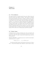
Figure 2.5.1: Impulse response, spectrum, covariogram, and
sample path of process (1 − .9L)y
t
= w
t
.
Y on X . The vector β is called the population least squares regression vector.
The law of large numbers for continuous state Markov processes Theorem 2.3.1
states conditions that guarantee that sample moments converge to population
moments, that is,
1
S


S
s=1
X

s
X
s
→ EX

X and
1
S

S
s=1
X

s
Y
s
→ EX

Y . Under
those conditions, sample least squares estimates converge to β.
There are as many such regressions as there are ways of selecting Y,X.
We have shown how a model (e.g., a triple A
o
,C,G, together with an initial
distribution for x

0
) restricts a regression. Going backward, that is, telling what
a given regression tells about a model, is more difficult. Often the regression
tells little about the model. The likelihood function encodes what a given data
set says about the model.
Population regression 49
0 10 20 30
0
0.2
0.4
0.6
0.8
1
impulse response
0 1 2 3
10
0
10
1
spectrum
−15 −10 −5 0 5 10 15
0
0.5
1
1.5
2
2.5
covariogram
20 40 60 80
−4

−3
−2
−1
0
1
2
3
sample path
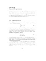
Figure 2.5.2: Impulse response, spectrum, covariogram, and
sample path of process (1 − .8L
4
)y
t
= w
t
.
2.5.1. The spectrum
For a covariance stationary stochastic process, all second moments can be en-
coded in a complex-valued matrix called the spectral density matrix. The auto-
covariance sequence for the process determines the spectral density. Conversely,
the spectral density can be used to determine the autocovariance sequence.
Under the assumption that A
o
is a stable matrix,
11
the state x
t
converges
to a unique covariance stationary probability distribution as t approaches infin-
ity. The spectral density matrix of this covariance stationary distribution S

x
(ω)
is defined to be the Fourier transform of the covariogram of x
t
:
S
x
(ω) ≡
∞

τ =−∞
C
x
(τ) e
−iωτ
. (2.5.5)
For the system (2.4.1), the spectral density of the stationary distribution is
given by the formula
S
x
(ω)=

I −A
o
e
−iω

−1
CC



I − A

o
e
+iω

−1
, ∀ω ∈ [−π, π] . (2.5.6)
11
It is sufficient that the only eigenvalue of A
o
not strictly less than unity in
modulus is that associated with the constant, which implies that A
o
and C fit
together in a way that validates (2.5.6).
50 Time series
0 10 20 30
−1
−0.5
0
0.5
1
1.5
impulse response
0 1 2 3
10
0
10

1
spectrum
−15 −10 −5 0 5 10 15
−1
0
1
2
3
4
covariogram
20 40 60 80
−4
−2
0
2
4
sample path
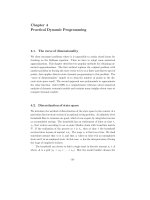
Figure 2.5.3: Impulse response, spectrum, covariogram, and
sample path of process (1 − 1.3L + .7L
2
)y
t
= w
t
.
The spectral density contains all of the information about the covariances. They
can be recovered from S
x
(ω) by the Fourier inversion formula
12

C
x
(τ)=(1/2π)

π
−π
S
x
(ω) e
+iωτ
dω.
Setting τ = 0 in the inversion formula gives
C
x
(0) = (1/2π)

π
−π
S
x
(ω) dω,
which shows that the spectral density decomposes covariance across frequen-
cies.
13
A formula used in the process of generalized method of moments (GMM)
estimation emerges by setting ω =0 inequation(2.5.5), which gives
S
x
(0) ≡
∞


τ =−∞
C
x
(τ) .
12
Spectral densities for continuous-time systems are discussed by Kwakernaak
and Sivan (1972). For an elementary discussion of discrete-time systems, see
Sargent (1987a). Also see Sargent (1987a, chap. 11) for definitions of the
spectral density function and methods of evaluating this integral.
13
More interestingly, the spectral density achieves a decomposition of covari-
ance into components that are orthogonal across frequencies.