Aircraft Flight Dynamics Robert F. Stengel Lecture15 Transfer Functions and Frequency Response
Bạn đang xem bản rút gọn của tài liệu. Xem và tải ngay bản đầy đủ của tài liệu tại đây (1.28 MB, 15 trang )
Transfer Functions and
Frequency Response
Robert Stengel, Aircraft Flight Dynamics
MAE 331, 2012"
• Frequency domain view of initial
condition response"
• Response of dynamic systems
to sinusoidal inputs"
• Transfer functions"
• Bode plots"
Copyright 2012 by Robert Stengel. All rights reserved. For educational use only.!
/>!
/>!
Laplace Transform of Initial
Condition Response
Laplace Transform of
a Dynamic System "
Δ
x(t ) = F Δx(t ) + G Δu(t) + LΔw(t )
• System equation!
• Laplace transform of system equation!
sΔx(s) − Δx(0) = F Δx(s ) + GΔ u(s) + LΔw(s)
dim(Δx) = (n × 1)
dim(Δu ) = (m × 1)
dim(Δw) = (s ×1)
Laplace Transform of
a Dynamic System "
• Rearrange Laplace transform of dynamic equation!
sΔx(s) − FΔ x(s) = Δx(0) + GΔ u(s) + LΔw(s)
sI − F
[ ]
Δx(s) = Δx(0) + GΔ u(s) + LΔw(s)
Δx(s) = sI − F
[ ]
−1
Δx(0) + G Δu(s) + LΔw(s)
[ ]
Initial !
Condition!
Control/Disturbance !
Input!
4
th
-Order Initial
Condition Response "
• Longitudinal dynamic model (time domain)!
Δx(s) = sI − F
[ ]
−1
Δx(0)
Δ
V (t)
Δ
γ
(t)
Δ
q(t)
Δ
α
(t)
$
%
&
&
&
&
&
'
(
)
)
)
)
)
=
−D
V
−g −D
q
−D
α
L
V
V
N
0
L
q
V
N
L
α
V
N
M
V
0 M
q
M
α
−
L
V
V
N
0 1 −
L
α
V
N
$
%
&
&
&
&
&
&
&
'
(
)
)
)
)
)
)
)
ΔV(t)
Δ
γ
(t)
Δq(t)
Δ
α
(t)
$
%
&
&
&
&
&
'
(
)
)
)
)
)
,
ΔV(0)
Δ
γ
(0)
Δq(0)
Δ
α
(0)
$
%
&
&
&
&
&
'
(
)
)
)
)
)
given
• Longitudinal model (frequency domain)!
ΔV(s)
Δ
γ
(s)
Δq(s)
Δ
α
(s)
$
%
&
&
&
&
&
'
(
)
)
)
)
)
= sI − F
Lon
[ ]
−1
ΔV(0)
Δ
γ
(0)
Δq(0)
Δ
α
(0)
$
%
&
&
&
&
&
'
(
)
)
)
)
)
Elements of the Characteristic
Matrix Inverse"
sI − F
Lon
≡ Δ
Lon
(s)
= s
4
+ a
3
s
3
+ a
2
s
2
+ a
1
s + a
0
Adj sI − F
Lon
( )
=
n
V
V
(s) n
γ
V
(s) n
q
V
(s) n
α
V
(s)
n
V
γ
(s) n
γ
γ
(s) n
q
γ
(s) n
α
γ
(s)
n
V
q
(s) n
γ
q
(s) n
q
q
(s) n
α
q
(s)
n
V
α
(s) n
V
α
(s) n
V
α
(s) n
V
α
(s)
$
%
&
&
&
&
&
&
'
(
)
)
)
)
)
)
sI − F
Lon
[ ]
−1
=
Adj sI − F
Lon
( )
sI − F
Lon
=
C
T
s
( )
Δ
Lon
(s)
(4 × 4)
1×1
( )
• Denominator
is scalar!
• Numerator is an (n x n) matrix of polynomials!
(sI – F)
–1
Distributes and Shapes the
Effects of Initial Conditions"
sI −F
Lon
[ ]
−1
=
n
V
V
(s) n
γ
V
(s) n
q
V
(s) n
α
V
(s)
n
V
γ
(s) n
γ
γ
(s) n
q
γ
(s) n
α
γ
(s)
n
V
q
(s) n
γ
q
(s) n
q
q
(s) n
α
q
(s)
n
V
α
(s) n
V
α
(s) n
V
α
(s) n
V
α
(s)
$
%
&
&
&
&
&
&
'
(
)
)
)
)
)
)
s
4
+ a
3
s
3
+ a
2
s
2
+ a
1
s + a
0
A
Lon
s
( )
(4 × 4)
1×1
( )
• Denominator determines the modes of motion"
• Numerator distributes each element of the initial
condition to each element of the state!
Δx(s) =
Adj sI −F
Lon
( )
sI − F
Lon
Δx(0) = A
Lon
s
( )
Δx(0) 4 ×1
( )
Relationship of (sI – F)
–1
to
State Transition Matrix, (t,0)"
• Initial condition response!
Δx(s) = sI − F
[ ]
−1
Δx(0) = A s
( )
Δx(0)
Δx(t ) = Φ t, 0
( )
Δx(0)
Time !
Domain!
Frequency !
Domain!
• Δx(s) is the Laplace transform of Δx(t)!
Δx(s) = A s
( )
Δx(0) = L Δx(t )
[ ]
= L Φ t,0
( )
Δx(0)
#
$
%
&
= L Φ t,0
( )
#
$
%
&
Δx(0)
Relationship of (sI – F)
–1
to
State Transition Matrix, (t,0)"
sI − F
[ ]
−1
= A s
( )
= L Φ t, 0
( )
#
$
%
&
= Laplace transform of the state transition matrix
• Therefore,!
Initial Condition Response of a
Single State Element "
A s
( )
sI − F
[ ]
−1
• Typical (ij
th
) element of A(s)!
a
ij
(s) =
k
ij
n
ij
(s)
Δ(s)
=
k
ij
s
q
+ b
q−1
s
q−1
+ +b
1
s + b
0
( )
s
n
+ a
n−1
s
n−1
+ + a
1
s + a
0
( )
=
k
ij
s − z
1
( )
ij
s − z
2
( )
ij
s − z
q
( )
ij
s −
λ
1
( )
s −
λ
2
( )
s −
λ
n
( )
Initial Condition Response of a
Single State Element "
p
i
(s) = k
i1
s
q
1
+ +b
0
( )
1
Δx
1
(0)++ k
in
s
q
n
+ +b
0
( )
n
Δx
n
(0)
k
p
i
s
q
max
+ + b
0
( )
• All terms have the same denominator polynomial"
• Terms sum to produce a single numerator polynomial!
Δx
i
(s) = a
i1
s
( )
Δx
1
(0)+ a
i2
s
( )
Δx
1
(0)++ a
in
s
( )
Δx
n
(0)
p
i
s
( )
Δ s
( )
• Initial condition response of Δx
i
(s)!
Real, scalar"
Partial Fraction Expansion of the
Initial Condition Response"
• Scalar response can be expressed with n parts,
each containing a single mode!
Δx
i
(s) =
p
i
s
( )
Δ s
( )
=
d
1
s −
λ
1
( )
+
d
2
s −
λ
2
( )
+
d
n
s −
λ
n
( )
$
%
&
&
'
(
)
)
i
, i =1,n
where, for each i, the (possibly complex) coefficients are
d
j
= s −
λ
j
( )
p
i
s
( )
Δ s
( )
s=
λ
j
, j = 1,n
Partial Fraction Expansion of the
Initial Condition Response"
• Time response is the inverse Laplace transform!
Δx
i
(t) = L
−1
Δx
i
(s)
[ ]
= L
−1
d
1
s −
λ
1
( )
+
d
2
s −
λ
2
( )
+
d
n
s −
λ
n
( )
$
%
&
'
(
)
i
= d
1
e
λ
1
t
+ d
2
e
λ
2
t
+ + d
n
e
λ
n
t
( )
i
, i = 1, n
Each element’s time response contains
every mode of the system (although
some coefficients may be zero)"
Scalar and Matrix
Transfer Functions
Response to a Control Input"
• Neglect initial condition"
• State response to control"
sΔx(s) = FΔx(s)+ GΔu(s)+ Δx(0), Δx(0) 0
Δx(s) = sI − F
[ ]
−1
G Δu(s)
• Output response to control"
Δy(s) = H
x
Δx(s)+H
u
Δu(s)
= H
x
sI − F
[ ]
−1
GΔu(s)+ H
u
Δu(s)
= H
x
sI − F
[ ]
−1
G + H
u
{ }
Δu(s)
Transfer Function Matrix"
• Frequency-domain effect of all inputs
on all outputs"
• Assume control effects do not appear
directly in the output: H
u
= 0"
• Transfer function matrix!
H (s) = H
x
sI − F
[ ]
−1
G H
x
A s
( )
G
r × n
( )
n × n
( )
n × m
( )
= r × m
( )
First-Order Transfer Function "
y s
( )
u s
( )
= H (s) = h s − f
[ ]
−1
g =
hg
s − f
( )
(n = m = r = 1)
• Scalar transfer function (= first-order lag)!
x t
( )
= fx t
( )
+ gu t
( )
y t
( )
= hx t
( )
• Scalar dynamic system!
Second-Order Transfer Function "
H(s) = H
x
A s
( )
G =
h
11
h
12
h
21
h
22
!
"
#
#
$
%
&
&
adj
s − f
11
( )
− f
12
− f
21
s − f
22
!
"
#
#
$
%
&
&
det
s − f
11
( )
− f
12
− f
21
s − f
22
( )
(
)
*
*
+
,
-
-
g
11
g
12
g
21
f
22
!
"
#
#
$
%
&
&
(n = m = r = 2)
• Second-order transfer function matrix!
r × n
( )
n × n
( )
n × m
( )
= r × m
( )
= 2 × 2
( )
x t
( )
=
x
1
t
( )
x
2
t
( )
!
"
#
#
$
%
&
&
=
f
11
f
12
f
21
f
22
!
"
#
#
$
%
&
&
x
1
t
( )
x
2
t
( )
!
"
#
#
$
%
&
&
+
g
11
g
12
g
21
f
22
!
"
#
#
$
%
&
&
u
1
t
( )
u
2
t
( )
!
"
#
#
$
%
&
&
y t
( )
=
y
1
t
( )
y
2
t
( )
!
"
#
#
$
%
&
&
=
h
11
h
12
h
21
h
22
!
"
#
#
$
%
&
&
x
1
t
( )
x
2
t
( )
!
"
#
#
$
%
&
&
• Second-order dynamic system!
Longitudinal Transfer
Function Matrix "
• With H
x
= I, and assuming"
– Elevator produces only a pitching moment"
– Throttle
affects only the rate of change of velocity"
– Flaps
produce only lift!
H
Lon
(s) = H
x
Lon
sI − F
Lon
[ ]
−1
G
Lon
= H
x
Lon
A
Lon
s
( )
G
Lon
=
1 0 0 0
0 1 0 0
0 0 1 0
0 0 0 1
"
#
$
$
$
$
%
&
'
'
'
'
n
V
V
(s) n
γ
V
(s) n
q
V
(s) n
α
V
(s)
n
V
γ
(s) n
γ
γ
(s) n
q
γ
(s) n
α
γ
(s)
n
V
q
(s) n
γ
q
(s) n
q
q
(s) n
α
q
(s)
n
V
α
(s) n
γ
α
(s) n
q
α
(s) n
α
α
(s)
"
#
$
$
$
$
$
$
%
&
'
'
'
'
'
'
0 T
δ
T
0
0 0 L
δ
F
/ V
N
M
δ
E
0 0
0 0 −L
δ
F
/ V
N
"
#
$
$
$
$
$
%
&
'
'
'
'
'
Δ
Lon
s
( )
Longitudinal Transfer
Function Matrix "
H
Lon
(s) =
n
δ
E
V
(s) n
δ
T
V
(s) n
δ
F
V
(s)
n
δ
E
γ
(s) n
δ
T
γ
(s) n
δ
F
γ
(s)
n
δ
E
q
(s) n
δ
T
q
(s) n
δ
F
q
(s)
n
δ
E
α
(s) n
δ
T
α
(s) n
δ
F
α
(s)
$
%
&
&
&
&
&
&
'
(
)
)
)
)
)
)
s
2
+ 2
ζ
P
ω
nP
s +
ω
n
P
2
( )
s
2
+ 2
ζ
SP
ω
n
SP
s +
ω
n
SP
2
( )
• There are 4 outputs and 3 inputs!
Douglas AD-1 Skyraider!
Longitudinal Transfer
Function Matrix "
ΔV(s)
Δ
γ
(s)
Δq(s)
Δ
α
(s)
$
%
&
&
&
&
&
'
(
)
)
)
)
)
= H
Lon
(s)
Δ
δ
E(s)
Δ
δ
T (s)
Δ
δ
F(s)
$
%
&
&
&
'
(
)
)
)
• Input-output relationship!
Scalar Transfer Function
from Δu
j
to Δy
i
"
H
ij
(s) =
k
ij
n
ij
(s)
Δ(s)
=
k
ij
s
q
+ b
q−1
s
q−1
+ + b
1
s + b
0
( )
s
n
+ a
n−1
s
n−1
+ + a
1
s + a
0
( )
# zeros = q!
# poles = n"
• Just one element of the matrix, H(s)"
• Denominator polynomial contains n roots"
• Each numerator term is a polynomial with q zeros,
where q varies from term to term and ≤ n – 1
!
=
k
ij
s − z
1
( )
ij
s − z
2
( )
ij
s − z
q
( )
ij
s −
λ
1
( )
s −
λ
2
( )
s −
λ
n
( )
Scalar Frequency Response
Function"
H
ij
(j
ω
) =
k
ij
j
ω
− z
1
( )
ij
j
ω
− z
2
( )
ij
j
ω
− z
q
( )
ij
j
ω
−
λ
1
( )
j
ω
−
λ
2
( )
j
ω
−
λ
n
( )
• Substitute: s = j
ω
!
• Frequency response is a complex function of
input frequency,
ω
"
– Real and imaginary parts, or"
– ** Amplitude ratio and phase angle **
!
= a(
ω
)+ jb(
ω
) → AR(
ω
) e
j
φ
(
ω
)
Transfer Function Matrix for
Short-Period Approximation "
• Transfer Function Matrix (with H
x
= I, H
u
= 0)"
H
SP
(s) = I
2
A
SP
s
( )
G
SP
=
s − M
q
( )
−M
α
− 1−
L
q
V
N
#
$
%
&
'
(
s +
L
α
V
N
( )
)
*
+
+
+
+
,
-
.
.
.
.
-1
M
δ
E
−L
δ
E
V
N
)
*
+
+
+
,
-
.
.
.
Δ
x
SP
=
Δ
q
Δ
α
#
$
%
%
&
'
(
(
≈
M
q
M
α
1 −
L
q
V
N
+
,
-
.
/
0
−
L
α
V
N
#
$
%
%
%
&
'
(
(
(
Δq
Δ
α
#
$
%
%
&
'
(
(
+
M
δ
E
−L
δ
E
V
N
#
$
%
%
%
&
'
(
(
(
Δ
δ
E
• Dynamic Equation"
Transfer Function Matrix for
Short-Period Approximation "
• Transfer Function Matrix (with H
x
= I, H
u
= 0)"
H
SP
(s ) = A
SP
s
( )
G
SP
=
s +
L
α
V
N
( )
M
α
1−
L
q
V
N
#
$
%
&
'
(
s − M
q
( )
)
*
+
+
+
+
,
-
.
.
.
.
M
δ
E
−L
δ
E
V
N
)
*
+
+
+
,
-
.
.
.
s − M
q
( )
s +
L
α
V
N
( )
− M
α
1−
L
q
V
N
#
$
%
&
'
(
Transfer Function Matrix for
Short-Period Approximation "
H
SP
(s) =
M
δ
E
s +
L
α
V
N
( )
−
L
δ
E
M
α
V
N
$
%
&
'
(
)
M
δ
E
1−
L
q
V
N
*
+
,
-
.
/
−
L
δ
E
V
N
( )
s − M
q
( )
$
%
&
'
(
)
$
%
&
&
&
&
&
'
(
)
)
)
)
)
s
2
+ −M
q
+
L
α
V
N
( )
s − M
α
1−
L
q
V
N
*
+
,
-
.
/
+ M
q
L
α
V
N
$
%
&
'
(
)
=
M
δ
E
s +
L
α
V
N
−
L
δ
E
M
α
V
N
M
δ
E
( )
$
%
&
'
(
)
−
L
δ
E
V
N
( )
s +
V
N
M
δ
E
L
δ
E
1−
L
q
V
N
*
+
,
-
.
/
− M
q
$
%
&
'
(
)
0
1
2
3
4
5
6
3
$
%
&
&
&
&
&
'
(
)
)
)
)
)
Δ
SP
s
( )
Transfer Function Matrix for
Short-Period Approximation "
H
SP
(s)
k
q
n
δ
E
q
(s)
k
α
n
δ
E
α
(s)
#
$
%
%
&
'
(
(
s
2
+ 2
ζ
SP
ω
n
SP
s +
ω
n
SP
2
=
Δq(s)
Δ
δ
E(s)
Δ
α
(s)
Δ
δ
E(s)
#
$
%
%
%
%
%
&
'
(
(
(
(
(
dim = 2 x 1"
Scalar Transfer
Functions for Short-
Period Approximation "
Δq(s)
Δ
δ
E(s)
=
M
δ
E
s +
L
α
V
N
−
L
δ
E
M
α
V
N
M
δ
E
( )
%
&
'
(
)
*
s
2
+ −M
q
+
L
α
V
N
( )
s − M
α
1 −
L
q
V
N
+
,
-
.
/
0
+ M
q
L
α
V
N
%
&
'
(
)
*
=
k
q
s − z
q
( )
s
2
+ 2
ζ
SP
ω
n
SP
s +
ω
n
SP
2
Δq(s)
Δ
α
(s)
#
$
%
%
&
'
(
(
=
Δq(s)
Δ
δ
E(s)
Δ
α
(s)
Δ
δ
E(s)
#
$
%
%
%
%
&
'
(
(
(
(
Δ
δ
E(s)
Δ
α
(s)
Δ
δ
E(s)
=
−
L
δ
E
V
N
( )
s +
V
N
M
δ
E
L
δ
E
1 −
L
q
V
N
%
&
'
(
)
*
− M
q
+
,
-
.
/
0
1
2
3
4
3
5
6
3
7
3
s
2
+ −M
q
+
L
α
V
N
( )
s − M
α
1 −
L
q
V
N
%
&
'
(
)
*
+ M
q
L
α
V
N
+
,
-
.
/
0
=
k
α
s − z
α
( )
s
2
+ 2
ζ
SP
ω
n
SP
s +
ω
n
SP
2
• Pitch Rate Transfer Function"
• Angle of Attack Transfer Function"
Short-Period Frequency Response (s = j
)
Expressed as Amplitude Ratio and Phase
Angle"
Pitch-rate frequency response"
Angle-of-attack frequency
response"
Δq( j
ω
)
Δ
δ
E( j
ω
)
=
k
q
j
ω
− z
q
( )
−
ω
2
+ 2
ζ
SP
ω
n
SP
j
ω
+
ω
n
SP
2
= AR
q
(
ω
) e
j
φ
q
(
ω
)
Δ
α
( j
ω
)
Δ
δ
E( j
ω
)
=
k
α
j
ω
− z
α
( )
−
ω
2
+ 2
ζ
SP
ω
n
SP
j
ω
+
ω
n
SP
2
= AR
α
(
ω
) e
j
φ
α
(
ω
)
Bode Plot
(Frequency Response of a
Scalar Transfer Function)
Angle and Rate
Response of a
DC Motor over
Wide Input-
Frequency
Range "
! Long-term response
of a dynamic system
to sinusoidal inputs
over a range of
frequencies"
! Determine
experimentally or "
! from the Bode plot
of the dynamic
system!
Very low damping!
Moderate damping!
High damping!
Bode Plot Portrays Response
to Sinusoidal Control Input"
• Express amplitude ratio in decibels
"
€
AR(dB) = 20log
10
AR original units
( )
[ ]
20 dB = factor of 10!
€
Δq( j
ω
)
Δ
δ
E( j
ω
)
=
k
q
j
ω
− z
q
( )
−
ω
2
+ 2
ζ
SP
ω
n
SP
j
ω
+
ω
n
SP
2
= AR
q
(
ω
) e
j
φ
q
(
ω
)
• Plot AR(dB) vs. log
10
(
ω
input
)"
• Plot phase angle,
ϕ
(deg) vs. log
10
(
ω
input
)"
• Asymptotes form “skeleton” of
response amplitude ratio"
• Asymptotes change at poles and zeros"
Products in original units
are sums in decibels!
# zeros = 1!
# poles = 2"
Constant Gain Bode Plot"
€
H( j
ω
) = 1
€
H( j
ω
) = 10
€
H( j
ω
) = 100
y t
( )
= hu t
( )
Slope = 0dB / dec, Amplitude Ratio = constant
Phase Angle = 0°
Integrator Bode Plot"
€
H( j
ω
) =
1
j
ω
€
H( j
ω
) =
10
j
ω
y t
( )
= h u t
( )
dt
0
t
∫
Slope = −20dB / dec
Phase Angle = −90°
Differentiator Bode Plot"
H ( j
ω
) = j
ω
€
H( j
ω
) =10 j
ω
y t
( )
= h
du t
( )
dt
Slope = +20dB / dec
Phase Angle = +90°
Sign Change"
H ( j
ω
) = −
h
j
ω
y t
( )
= −h u t
( )
dt
0
t
∫
H ( j
ω
) = − j
ω
y t
( )
= −h
du t
( )
dt
Slope = −20dB / dec
Phase Angle = +90°
Slope = +20dB / dec
Phase Angle = −90°
Integral!
Derivative!
Multiple Integrators and
Differentiators"
H ( j
ω
) = h j
ω
( )
2
y t
( )
= h
d
2
u t
( )
dt
2
H ( j
ω
) =
h
j
ω
( )
2
y t
( )
= h u t
( )
dt
2
0
t
∫
0
t
∫
Slope = −40dB / dec
Phase Angle = −180°
Slope = +40dB / dec
Phase Angle = +180°
Double Integral!
Double Derivative!
Constant Gain, Integrator, and
Differentiator Bode Plots Form the
Asymptotes for More Complex
Transfer Functions"
+20 "
dB/dec"
+40 "
dB/dec"
0 "
dB/dec"
+20 "
dB/dec"
–20 "
dB/dec"
Bode Plots of First-Order Lags"
H
red
( j
ω
) =
10
j
ω
+10
( )
H
blue
( j
ω
) =
100
j
ω
+10
( )
H
green
( j
ω
) =
100
j
ω
+100
( )
Bode Plot Asymptotes, Departures,
and Phase Angles for First-Order Lags"
• General shape of amplitude
ratio governed by
asymptotes"
• Slope of asymptotes
changes by multiples of ±20
dB/dec at poles or zeros"
• Actual AR departs from
asymptotes"
• Phase angle of a real,
negative pole"
– When
ω
= 0,
ϕ
= 0°"
– When
ω
=
λ
,
ϕ
=–45°"
– When ω -> ∞,
ϕ
-> –90°"
• AR asymptotes of a real pole"
– When
ω
= 0, slope = 0 dB/
dec"
– When
ω
≥
λ
, slope = –20 dB/
dec"
Bode Plots of Second-Order Lags
(No Zeros)"
Effect of
Damping Ratio!
H
green
( j
ω
) =
10
2
j
ω
( )
2
+ 2 0.1
( )
10
( )
j
ω
( )
+10
2
H
blue
( j
ω
) =
10
2
j
ω
( )
2
+ 2 0.4
( )
10
( )
j
ω
( )
+10
2
H
red
( j
ω
) =
10
2
j
ω
( )
2
+ 2 0.707
( )
10
( )
j
ω
( )
+10
2
Bode Plots of Second-Order Lags
(No Zeros)"
H
red
( j
ω
) =
10
2
j
ω
( )
2
+ 2 0.1
( )
10
( )
j
ω
( )
+10
2
Effects of Gain and
Natural Frequency!
H
green
( j
ω
) =
10
3
j
ω
( )
2
+ 2 0.1
( )
10
( )
j
ω
( )
+10
2
H
blue
( j
ω
) =
100
2
j
ω
( )
2
+ 2 0.1
( )
100
( )
j
ω
( )
+100
2
Amplitude Ratio Asymptotes and Departures of
Second-Order Bode Plots (No Zeros)"
• AR asymptotes of a
pair of complex poles"
– When
ω
= 0, slope
= 0 dB/dec"
– When
ω
≥
ω
n
,
slope = –40 dB/
dec"
• Height of resonant
peak depends on
damping ratio"
Phase Angles of Second-Order
Bode Plots (No Zeros)"
• Phase angle of a pair
of complex negative
poles"
– When
ω
= 0,
ϕ
= 0°"
– When
ω
=
ω
n
,
ϕ
=–
90°"
– When
ω
-> ∞,
ϕ
-> –
180°"
• Abruptness of phase
shift depends on
damping ratio"
MATLAB Bode Plot with asymp.m"
/> />2
nd
-Order Pitch Rate Frequency Response"
asymp.m"bode.m"
Frequency
Response AR
Departures in the
Vicinity of Poles"
• Difference between
actual amplitude ratio
(dB) and asymptote =
departure (dB)"
• Results for multiple roots
are additive"
• from McRuer, Ashkenas,
and Graham, Aircraft
Dynamics and Automatic
Control, Princeton
University Press, 1973"
• Zero departures have
opposite sign"
First- and Second-Order Departures
from Amplitude Ratio Asymptotes"
First- and Second-
Order Phase Angles"
Phase Angle
Variations in the
Vicinity of Poles"
• Results for multiple roots
are additive"
• from McRuer, Ashkenas,
and Graham, Aircraft
Dynamics and Automatic
Control, Princeton
University Press, 1973"
• LHP zero variations have
opposite sign"
• RHP zeros have same
sign"
Next Time:
Control Devices and Systems
Reading
Flight Dynamics, 214-234
Virtual Textbook, Part 16
Supplementary
Material
Bode Plots of 1
st
- and 2
nd
-Order Lags"
€
H
red
( j
ω
) =
10
j
ω
+ 10
( )
H
blue
( j
ω
) =
100
2
j
ω
( )
2
+ 2 0.1
( )
100
( )
j
ω
( )
+ 100
2
Bode Plots of 3
rd
-Order Lags"
€
H
blue
( j
ω
) =
10
j
ω
+ 10
( )
#
$
%
&
'
(
100
2
j
ω
( )
2
+ 2 0.1
( )
100
( )
j
ω
( )
+ 100
2
#
$
%
%
&
'
(
(
H
green
( j
ω
) =
10
2
j
ω
( )
2
+ 2 0.1
( )
10
( )
j
ω
( )
+ 10
2
#
$
%
%
&
'
(
(
100
j
ω
+ 100
( )
#
$
%
&
'
(
Bode Plot of a 4
th
-Order System with
No Zeros"
H ( j
ω
) =
1
2
j
ω
( )
2
+ 2 0.05
( )
1
( )
j
ω
( )
+ 1
2
"
#
$
$
%
&
'
'
100
2
j
ω
( )
2
+ 2 0.1
( )
100
( )
j
ω
( )
+ 100
2
"
#
$
$
%
&
'
'
• Resonant peaks and
large phase shifts at
each natural frequency"
• Additive AR slope shifts
at each natural
frequency"
# zeros = 0!
# poles = 4"
Left-Half-Plane Transfer Function Zero"
H ( j
ω
) = j
ω
+ 10
( )
• Zeros are numerator singularities "
H (j
ω
) =
k j
ω
− z
1
( )
j
ω
− z
2
( )
j
ω
−
λ
1
( )
j
ω
−
λ
2
( )
j
ω
−
λ
n
( )
• Single zero in left half
plane"
• Introduces a +20 dB/
dec slope"
• Produces phase lead
in vicinity of zero"
Right-Half-Plane Transfer Function Zero"
H ( j
ω
) = − j
ω
− 10
( )
• Single zero in right half
plane"
• Introduces a +20 dB/dec
slope"
• Produces phase lag in
vicinity of zero"
Second-Order Transfer Function Zero"
€
H( j
ω
) = j
ω
− z
( )
j
ω
− z
*
( )
= j
ω
( )
2
+ 2 0.1
( )
100
( )
j
ω
( )
+ 100
2
[ ]
• Complex pair of
zeros produces an
amplitude ratio
notch at its
natural frequency"
4
th
-Order Transfer Function with
2
nd
-Order Zero"
€
H( j
ω
) =
j
ω
( )
2
+ 2 0.1
( )
10
( )
j
ω
( )
+ 10
2
[ ]
j
ω
( )
2
+ 2 0.05
( )
1
( )
j
ω
( )
+ 1
2
[ ]
j
ω
( )
2
+ 2 0.1
( )
100
( )
j
ω
( )
+ 100
2
[ ]
Elevator-to-
Normal-Velocity
Frequency
Response"
Δw(s)
Δ
δ
E(s)
=
n
δ
E
w
(s)
Δ
Lon
(s)
≈
M
δ
E
s
2
+ 2
ζω
n
s +
ω
n
2
( )
Approx Ph
s − z
3
( )
s
2
+ 2
ζω
n
s +
ω
n
2
( )
Ph
s
2
+ 2
ζω
n
s +
ω
n
2
( )
SP
0 dB/dec!
+40 dB/dec!
0 dB/dec!
–40 dB/dec!
–20 dB/dec!
• (n – q) = 1"
• Complex zero
almost (but
not quite)
cancels
phugoid
response
"
Short "
Period"
Phugoid"