OpenGL Programming Guide potx

OpenGL Programming Guide
About This Guide
The OpenGL graphics system is a software interface to graphics hardware. (The GL stands for
Graphics Library.) It allows you to create interactive programs that produce color images of moving
three−dimensional objects. With OpenGL, you can control computer−graphics technology to produce
realistic pictures or ones that depart from reality in imaginative ways. This guide explains how to
program with the OpenGL graphics system to deliver the visual effect you want.
What This Guide Contains
This guide has the ideal number of chapters: 13. The first six chapters present basic information that
you need to understand to be able to draw a properly colored and lit three−dimensional object on the
screen:
• Chapter 1, "Introduction to OpenGL," provides a glimpse into the kinds of things OpenGL can
do. It also presents a simple OpenGL program and explains essential programming details you
need to know for subsequent chapters.
• Chapter 2, "Drawing Geometric Objects," explains how to create a three−dimensional
geometric description of an object that is eventually drawn on the screen.
• Chapter 3, "Viewing," describes how such three−dimensional models are transformed before being
drawn onto a two−dimensional screen. You can control these transformations to show a particular
view of a model.
• Chapter 4, "Display Lists," discusses how to store a series of OpenGL commands for execution at
a later time. You’ll want to use this feature to increase the performance of your OpenGL program.
• Chapter 5, "Color," describes how to specify the color and shading method used to draw an object.
• Chapter 6, "Lighting," explains how to control the lighting conditions surrounding an object and
how that object responds to light (that is, how it reflects or absorbs light). Lighting is an important
topic, since objects usually don’t look three−dimensional until they’re lit.
The remaining chapters explain how to add sophisticated features to your three−dimensional scene.
You might choose not to take advantage of many of these features until you’re more comfortable with
OpenGL. Particularly advanced topics are noted in the text where they occur.
• Chapter 7, "Blending, Antialiasing, and Fog," describes techniques essential to creating a
realistic scenealpha blending (which allows you to create transparent objects), antialiasing, and
atmospheric effects (such as fog or smog).

• Chapter 8, "Drawing Pixels, Bitmaps, Fonts, and Images," discusses how to work with sets of
two−dimensional data as bitmaps or images. One typical use for bitmaps is to describe characters
in fonts.
• Chapter 9, "Texture Mapping," explains how to map one− and two−dimensional images called
textures onto three−dimensional objects. Many marvelous effects can be achieved through texture
mapping.
• Chapter 10, "The Framebuffer," describes all the possible buffers that can exist in an OpenGL
implementation and how you can control them. You can use the buffers for such effects as
hidden−surface elimination, stenciling, masking, motion blur, and depth−of−field focusing.
• Chapter 11, "Evaluators and NURBS," gives an introduction to advanced techniques for
efficiently generating curves or surfaces.
• Chapter 12, "Selection and Feedback," explains how you can use OpenGL’s selection
mechanism to select an object on the screen. It also explains the feedback mechanism, which allows
you to collect the drawing information OpenGL produces rather than having it be used to draw on
the screen.
1
• Chapter 13, "Now That You Know," describes how to use OpenGL in several clever and
unexpected ways to produce interesting results. These techniques are drawn from years of
experience with the technological precursor to OpenGL, the Silicon Graphics IRIS Graphics
Library.
In addition, there are several appendices that you will likely find useful:
• Appendix A, "Order of Operations," gives a technical overview of the operations OpenGL
performs, briefly describing them in the order in which they occur as an application executes.
• Appendix B, "OpenGL State Variables," lists the state variables that OpenGL maintains and
describes how to obtain their values.
• Appendix C, "The OpenGL Utility Library," briefly describes the routines available in the
OpenGL Utility Library.
• Appendix D, "The OpenGL Extension to the X Window System," briefly describes the
routines available in the OpenGL extension to the X Window System.
• Appendix E, "The OpenGL Programming Guide Auxiliary Library," discusses a small C code

library that was written for this book to make code examples shorter and more comprehensible.
• Appendix F, "Calculating Normal Vectors," tells you how to calculate normal vectors for
different types of geometric objects.
• Appendix G, "Homogeneous Coordinates and Transformation Matrices," explains some of
the mathematics behind matrix transformations.
• Appendix H, "Programming Tips," lists some programming tips based on the intentions of the
designers of OpenGL that you might find useful.
• Appendix I, "OpenGL Invariance," describes the pixel−exact invariance rules that OpenGL
implementations follow.
• Appendix J, "Color Plates," contains the color plates that appear in the printed version of this
guide.
Finally, an extensive Glossary defines the key terms used in this guide.
How to Obtain the Sample Code
This guide contains many sample programs to illustrate the use of particular OpenGL programming
techniques. These programs make use of a small auxiliary library that was written for this guide. The
section "OpenGL−related Libraries" gives more information about this auxiliary library. You can
obtain the source code for both the sample programs and the auxiliary library for free via ftp
(file−transfer protocol) if you have access to the Internet.
First, use ftp to go to the host sgigate.sgi.com, and use anonymous as your user name and your_name@
machine as the password. Then type the following:
cd pub/opengl
binary
get opengl.tar.Z
bye
The file you receive is a compressed tar archive. To restore the files, type:
uncompress opengl.tar
tar xf opengl.tar
The sample programs and auxiliary library are created as subdirectories from wherever you are in the
file directory structure.
Many implementations of OpenGL might also include the code samples and auxiliary library as part of

the system. This source code is probably the best source for your implementation, because it might have
been optimized for your system. Read your machine−specific OpenGL documentation to see where the
code samples can be found.
2
What You Should Know Before Reading This Guide
This guide assumes only that you know how to program in the C language and that you have some
background in mathematics (geometry, trigonometry, linear algebra, calculus, and differential
geometry). Even if you have little or no experience with computer−graphics technology, you should be
able to follow most of the discussions in this book. Of course, computer graphics is a huge subject, so
you may want to enrich your learning experience with supplemental reading:
• Computer Graphics: Principles and Practice by James D. Foley, Andries van Dam, Steven K.
Feiner, and John F. Hughes (Reading, Mass.: Addison−Wesley Publishing Co.)This book is an
encyclopedic treatment of the subject of computer graphics. It includes a wealth of information but
is probably best read after you have some experience with the subject.
• 3D Computer Graphics: A User’s Guide for Artists and Designers by Andrew S. Glassner (New York:
Design Press)This book is a nontechnical, gentle introduction to computer graphics. It focuses on
the visual effects that can be achieved rather than on the techniques needed to achieve them.
Once you begin programming with OpenGL, you might want to obtain the OpenGL Reference Manual
by the OpenGL Architecture Review Board (Reading, Mass.: Addison−Wesley Publishing Co., 1993),
which is designed as a companion volume to this guide. The Reference Manual provides a technical
view of how OpenGL operates on data that describes a geometric object or an image to produce an
image on the screen. It also contains full descriptions of each set of related OpenGL commandsthe
parameters used by the commands, the default values for those parameters, and what the commands
accomplish.
"OpenGL" is really a hardware−independent specification of a programming interface. You use a
particular implementation of it on a particular kind of hardware. This guide explains how to program
with any OpenGL implementation. However, since implementations may vary slightlyin performance
and in providing additional, optional features, for exampleyou might want to investigate whether
supplementary documentation is available for the particular implementation you’re using. In addition,
you might have OpenGL−related utilities, toolkits, programming and debugging support, widgets,

sample programs, and demos available to you with your system.
Style Conventions
These style conventions are used in this guide:
• BoldCommand and routine names, and matrices
• ItalicsVariables, arguments, parameter names, spatial dimensions, and matrix components
• RegularEnumerated types and defined constants
Code examples are set off from the text in a monospace font, and command summaries are shaded with
gray boxes.
Topics that are particularly complicatedand that you can skip if you’re new to OpenGL or computer
graphicsare marked with the Advanced icon. This icon can apply to a single paragraph or to an entire
section or chapter.
Advanced
Exercises that are left for the reader are marked with the Try This icon.
Try This
Acknowledgments
No book comes into being without the help of many people. Probably the largest debt the authors owe is
to the creators of OpenGL itself. The OpenGL team at Silicon Graphics has been led by Kurt Akeley,
3
Bill Glazier, Kipp Hickman, Phil Karlton, Mark Segal, Kevin P. Smith, and Wei Yen. The members of
the OpenGL Architecture Review Board naturally need to be counted among the designers of OpenGL:
Dick Coulter and John Dennis of Digital Equipment Corporation; Jim Bushnell and Linas Vepstas of
International Business Machines, Corp.; Murali Sundaresan and Rick Hodgson of Intel; and On Lee
and Chuck Whitmore of Microsoft. Other early contributors to the design of OpenGL include Raymond
Drewry of Gain Technology, Inc., Fred Fisher of Digital Equipment Corporation, and Randi Rost of
Kubota Pacific Computer, Inc. Many other Silicon Graphics employees helped refine the definition and
functionality of OpenGL, including Momi Akeley, Allen Akin, Chris Frazier, Paul Ho, Simon Hui,
Lesley Kalmin, Pierre Tardiff, and Jim Winget.
Many brave souls volunteered to review this book: Kurt Akeley, Gavin Bell, Sam Chen, Andrew
Cherenson, Dan Fink, Beth Fryer, Gretchen Helms, David Marsland, Jeanne Rich, Mark Segal, Kevin
P. Smith, and Josie Wernecke from Silicon Graphics; David Niguidula, Coalition of Essential Schools,

Brown University; John Dennis and Andy Vesper, Digital Equipment Corporation; Chandrasekhar
Narayanaswami and Linas Vepstas, International Business Machines, Corp.; Randi Rost, Kubota
Pacific; On Lee, Microsoft Corp.; Dan Sears; Henry McGilton, Trilithon Software; and Paula Womak.
Assembling the set of colorplates was no mean feat. The sequence of plates based on the cover image (
Figure J−1 through Figure J−9 ) was created by Thad Beier of Pacific Data Images, Seth Katz of
Xaos Tools, Inc., and Mason Woo of Silicon Graphics. Figure J−10 through Figure J−32 are
snapshots of programs created by Mason. Gavin Bell, Kevin Goldsmith, Linda Roy, and Mark Daly (all
of Silicon Graphics) created the fly−through program used for Figure J−34 . The model for Figure
J−35 was created by Barry Brouillette of Silicon Graphics; Doug Voorhies, also of Silicon Graphics,
performed some image processing for the final image. Figure J−36 was created by John Rohlf and
Michael Jones, both of Silicon Graphics. Figure J−37 was created by Carl Korobkin of Silicon
Graphics. Figure J−38 is a snapshot from a program written by Gavin Bell with contributions from
the Inventor team at Silicon GraphicsAlain Dumesny, Dave Immel, David Mott, Howard Look, Paul
Isaacs, Paul Strauss, and Rikk Carey. Figure J−39 and Figure J−40 are snapshots from a visual
simulation program created by the Silicon Graphics IRIS Performer teamCraig Phillips, John Rohlf,
Sharon Fischler, Jim Helman, and Michael Jonesfrom a database produced for Silicon Graphics by
Paradigm Simulation, Inc. Figure J−41 is a snapshot from skyfly, the precursor to Performer, which
was created by John Rohlf, Sharon Fischler, and Ben Garlick, all of Silicon Graphics.
Several other people played special roles in creating this book. If we were to list other names as authors
on the front of this book, Kurt Akeley and Mark Segal would be there, as honorary yeoman. They
helped define the structure and goals of the book, provided key sections of material for it, reviewed it
when everybody else was too tired of it to do so, and supplied that all−important humor and support
throughout the process. Kay Maitz provided invaluable production and design assistance. Kathy
Gochenour very generously created many of the illustrations for this book. Tanya Kucak copyedited the
manuscript, in her usual thorough and professional style.
And now, each of the authors would like to take the 15 minutes that have been allotted to them by
Andy Warhol to say thank you.
I’d like to thank my managers at Silicon GraphicsDave Larson and Way Tingand the members of
my groupPatricia Creek, Arthur Evans, Beth Fryer, Jed Hartman, Ken Jones, Robert Reimann, Eve
Stratton (aka Margaret−Anne Halse), John Stearns, and Josie Werneckefor their support during this

lengthy process. Last but surely not least, I want to thank those whose contributions toward this
project are too deep and mysterious to elucidate: Yvonne Leach, Kathleen Lancaster, Caroline Rose,
Cindy Kleinfeld, and my parents, Florence and Ferdinand Neider.
JLN
In addition to my parents, Edward and Irene Davis, I’d like to thank the people who taught me most of
what I know about computers and computer graphicsDoug Engelbart and Jim Clark.
TRD
I’d like to thank the many past and current members of Silicon Graphics whose accommodation and
4
enlightenment were essential to my contribution to this book: Gerald Anderson, Wendy Chin, Bert
Fornaciari, Bill Glazier, Jill Huchital, Howard Look, Bill Mannel, David Marsland, Dave Orton, Linda
Roy, Keith Seto, and Dave Shreiner. Very special thanks to Karrin Nicol and Leilani Gayles of SGI for
their guidance throughout my career. I also bestow much gratitude to my teammates on the Stanford B
ice hockey team for periods of glorious distraction throughout the writing of this book. Finally, I’d like
to thank my family, especially my mother, Bo, and my late father, Henry.
MW
Chapter 1
Introduction to OpenGL
Chapter Objectives
After reading this chapter, you’ll be able to do the following:
• Appreciate in general terms what OpenGL offers
• Identify different levels of rendering complexity
• Understand the basic structure of an OpenGL program
• Recognize OpenGL command syntax
• Understand in general terms how to animate an OpenGL program
This chapter introduces OpenGL. It has the following major sections:
• "What Is OpenGL?" explains what OpenGL is, what it does and doesn’t do, and how it works.
• "A Very Simple OpenGL Program" presents a small OpenGL program and briefly discusses it.
This section also defines a few basic computer−graphics terms.
• "OpenGL Command Syntax" explains some of the conventions and notations used by OpenGL

commands.
• "OpenGL as a State Machine" describes the use of state variables in OpenGL and the commands
for querying, enabling, and disabling states.
• "OpenGL−related Libraries" describes sets of OpenGL−related routines, including an auxiliary
library specifically written for this book to simplify programming examples.
• "Animation" explains in general terms how to create pictures on the screen that move, or animate.
What Is OpenGL?
OpenGL is a software interface to graphics hardware. This interface consists of about 120 distinct
commands, which you use to specify the objects and operations needed to produce interactive
three−dimensional applications.
OpenGL is designed to work efficiently even if the computer that displays the graphics you create isn’t
the computer that runs your graphics program. This might be the case if you work in a networked
computer environment where many computers are connected to one another by wires capable of
carrying digital data. In this situation, the computer on which your program runs and issues OpenGL
drawing commands is called the client, and the computer that receives those commands and performs
the drawing is called the server. The format for transmitting OpenGL commands (called the protocol)
from the client to the server is always the same, so OpenGL programs can work across a network even
if the client and server are different kinds of computers. If an OpenGL program isn’t running across a
network, then there’s only one computer, and it is both the client and the server.
OpenGL is designed as a streamlined, hardware−independent interface to be implemented on many
different hardware platforms. To achieve these qualities, no commands for performing windowing tasks
or obtaining user input are included in OpenGL; instead, you must work through whatever windowing
system controls the particular hardware you’re using. Similarly, OpenGL doesn’t provide high−level
commands for describing models of three−dimensional objects. Such commands might allow you to
specify relatively complicated shapes such as automobiles, parts of the body, airplanes, or molecules.
5
With OpenGL, you must build up your desired model from a small set of geometric primitivepoints,
lines, and polygons. (A sophisticated library that provides these features could certainly be built on top
of OpenGLin fact, that’s what Open Inventor is. See "OpenGL−related Libraries" for more
information about Open Inventor.)

Now that you know what OpenGL doesn’t do, here’s what it does do. Take a look at the color plates
they illustrate typical uses of OpenGL. They show the scene on the cover of this book, drawn by a
computer (which is to say, rendered) in successively more complicated ways. The following paragraphs
describe in general terms how these pictures were made.
• Figure J−1 shows the entire scene displayed as a wireframe modelthat is, as if all the objects in
the scene were made of wire. Each line of wire corresponds to an edge of a primitive (typically a
polygon). For example, the surface of the table is constructed from triangular polygons that are
positioned like slices of pie.
Note that you can see portions of objects that would be obscured if the objects were solid rather
than wireframe. For example, you can see the entire model of the hills outside the window even
though most of this model is normally hidden by the wall of the room. The globe appears to be
nearly solid because it’s composed of hundreds of colored blocks, and you see the wireframe lines for
all the edges of all the blocks, even those forming the back side of the globe. The way the globe is
constructed gives you an idea of how complex objects can be created by assembling lower−level
objects.
• Figure J−2 shows a depth−cued version of the same wireframe scene. Note that the lines farther
from the eye are dimmer, just as they would be in real life, thereby giving a visual cue of depth.
• Figure J−3 shows an antialiased version of the wireframe scene. Antialiasing is a technique for
reducing the jagged effect created when only portions of neighboring pixels properly belong to the
image being drawn. Such jaggies are usually the most visible with near−horizontal or near−vertical
lines.
• Figure J−4 shows a flat−shaded version of the scene. The objects in the scene are now shown as
solid objects of a single color. They appear "flat" in the sense that they don’t seem to respond to the
lighting conditions in the room, so they don’t appear smoothly rounded.
• Figure J−5 shows a lit, smooth−shaded version of the scene. Note how the scene looks much more
realistic and three−dimensional when the objects are shaded to respond to the light sources in the
room; the surfaces of the objects now look smoothly rounded.
• Figure J−6 adds shadows and textures to the previous version of the scene. Shadows aren’t an
explicitly defined feature of OpenGL (there is no "shadow command"), but you can create them
yourself using the techniques described in Chapter 13 . Texture mapping allows you to apply a

two−dimensional texture to a three−dimensional object. In this scene, the top on the table surface is
the most vibrant example of texture mapping. The walls, floor, table surface, and top (on top of the
table) are all texture mapped.
• Figure J−7 shows a motion−blurred object in the scene. The sphinx (or dog, depending on your
Rorschach tendencies) appears to be captured as it’s moving forward, leaving a blurred trace of its
path of motion.
• Figure J−8 shows the scene as it’s drawn for the cover of the book from a different viewpoint. This
plate illustrates that the image really is a snapshot of models of three−dimensional objects.
The next two color images illustrate yet more complicated visual effects that can be achieved with
OpenGL:
• Figure J−9 illustrates the use of atmospheric effects (collectively referred to as fog) to show the
presence of particles in the air.
• Figure J−10 shows the depth−of−field effect, which simulates the inability of a camera lens to
maintain all objects in a photographed scene in focus. The camera focuses on a particular spot in
the scene, and objects that are significantly closer or farther than that spot are somewhat blurred.
The color plates give you an idea of the kinds of things you can do with the OpenGL graphics system.
The next several paragraphs briefly describe the order in which OpenGL performs the major graphics
operations necessary to render an image on the screen. Appendix A, "Order of Operations"
describes this order of operations in more detail.
6

Giáo trình AutoCad 2004









1. Construct shapes from geometric primitives, thereby creating mathematical descriptions of objects.
(OpenGL considers points, lines, polygons, images, and bitmaps to be primitives.)
2. Arrange the objects in three−dimensional space and select the desired vantage point for viewing the
composed scene.
3. Calculate the color of all the objects. The color might be explicitly assigned by the application,
determined from specified lighting conditions, or obtained by pasting a texture onto the objects.
4. Convert the mathematical description of objects and their associated color information to pixels on
the screen. This process is called rasterization.
During these stages, OpenGL might perform other operations, such as eliminating parts of objects that
are hidden by other objects (the hidden parts won’t be drawn, which might increase performance). In
addition, after the scene is rasterized but just before it’s drawn on the screen, you can manipulate the
pixel data if you want.
A Very Simple OpenGL Program
Because you can do so many things with the OpenGL graphics system, an OpenGL program can be
complicated. However, the basic structure of a useful program can be simple: Its tasks are to initialize
certain states that control how OpenGL renders and to specify objects to be rendered.
Before you look at an OpenGL program, let’s go over a few terms. Rendering, which you’ve already seen
used, is the process by which a computer creates images from models. These models, or objects, are
constructed from geometric primitivespoints, lines, and polygonsthat are specified by their vertices.
The final rendered image consists of pixels drawn on the screen; a pixelshort for picture elementis

the smallest visible element the display hardware can put on the screen. Information about the pixels
(for instance, what color they’re supposed to be) is organized in system memory into bitplanes. A
bitplane is an area of memory that holds one bit of information for every pixel on the screen; the bit
might indicate how red a particular pixel is supposed to be, for example. The bitplanes are themselves
organized into a framebuffer, which holds all the information that the graphics display needs to control
the intensity of all the pixels on the screen.
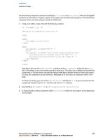
Now look at an OpenGL program. Example 1−1 renders a white rectangle on a black background, as
shown in Figure 1−1 .
7
Figure 1−1 A White Rectangle on a Black Background
Example 1−1 A Simple OpenGL Program
#include <whateverYouNeed.h>
main() {
OpenAWindowPlease();
glClearColor(0.0, 0.0, 0.0, 0.0);
glClear(GL_COLOR_BUFFER_BIT);
glColor3f(1.0, 1.0, 1.0);
glOrtho(−1.0, 1.0, −1.0, 1.0, −1.0, 1.0);
glBegin(GL_POLYGON);
glVertex2f(−0.5, −0.5);
glVertex2f(−0.5, 0.5);
glVertex2f(0.5, 0.5);
glVertex2f(0.5, −0.5);
glEnd();
glFlush();
KeepTheWindowOnTheScreenForAWhile();
}
The first line of the main() routine opens a window on the screen: The OpenAWindowPlease() routine is
meant as a placeholder for a window system−specific routine. The next two lines are OpenGL
commands that clear the window to black: glClearColor() establishes what color the window will be

cleared to, and glClear() actually clears the window. Once the color to clear to is set, the window is
8
cleared to, and glClear() actually clears the window. Once the color to clear to is set, the window is
cleared to that color whenever glClear() is called. The clearing color can be changed with another call to
glClearColor(). Similarly, the glColor3f() command establishes what color to use for drawing objects
in this case, the color is white. All objects drawn after this point use this color, until it’s changed with
another call to set the color.
The next OpenGL command used in the program, glOrtho(), specifies the coordinate system OpenGL
assumes as it draws the final image and how the image gets mapped to the screen. The next calls,
which are bracketed by glBegin() and glEnd(), define the object to be drawnin this example, a polygon
with four vertices. The polygon’s "corners" are defined by the glVertex2f() commands. As you might be
able to guess from the arguments, which are (x, y) coordinate pairs, the polygon is a rectangle.
Finally, glFlush() ensures that the drawing commands are actually executed, rather than stored in a
buffer awaiting additional OpenGL commands. The KeepTheWindowOnTheScreenForAWhile()
placeholder routine forces the picture to remain on the screen instead of immediately disappearing.
OpenGL Command Syntax
As you might have observed from the simple program in the previous section, OpenGL commands use
the prefix gl and initial capital letters for each word making up the command name (recall
glClearColor(), for example). Similarly, OpenGL defined constants begin with GL_, use all capital
letters, and use underscores to separate words (like GL_COLOR_BUFFER_BIT).
You might also have noticed some seemingly extraneous letters appended to some command names
(the 3f in glColor3f(), for example). It’s true that the Color part of the command name is enough to
define the command as one that sets the current color. However, more than one such command has
been defined so that you can use different types of arguments. In particular, the 3 part of the suffix
indicates that three arguments are given; another version of the Color command takes four arguments.
The f part of the suffix indicates that the arguments are floating−point numbers. Some OpenGL
commands accept as many as eight different data types for their arguments. The letters used as
suffixes to specify these data types for ANSI C implementations of OpenGL are shown in Table 1−1 ,
along with the corresponding OpenGL type definitions. The particular implementation of OpenGL that
you’re using might not follow this scheme exactly; an implementation in C++ or Ada, for example,

wouldn’t need to.
SuffixData Type Typical Corresponding
C−Language Type
OpenGL Type Definition
b 8−bit integer signed char GLbyte
s 16−bit integer short GLshort
i 32−bit integer long GLint, GLsizei
f 32−bit floating−point float GLfloat, GLclampf
d 64−bit floating−point double GLdouble, GLclampd
ub 8−bit unsigned integer unsigned char GLubyte, GLboolean
us 16−bit unsigned integer unsigned short GLushort
ui 32−bit unsigned integer unsigned long GLuint, GLenum, GLbitfield
Table 1−1 Command Suffixes and Argument Data Types
Thus, the two commands
glVertex2i(1, 3);
glVertex2f(1.0, 3.0);
are equivalent, except that the first specifies the vertex’s coordinates as 32−bit integers and the second
specifies them as single−precision floating−point numbers.
Some OpenGL commands can take a final letter v, which indicates that the command takes a pointer to
a vector (or array) of values rather than a series of individual arguments. Many commands have both
vector and nonvector versions, but some commands accept only individual arguments and others
9
vector and nonvector versions, but some commands accept only individual arguments and others
require that at least some of the arguments be specified as a vector. The following lines show how you
might use a vector and a nonvector version of the command that sets the current color:
glColor3f(1.0, 0.0, 0.0);
float color_array[] = {1.0, 0.0, 0.0};
glColor3fv(color_array);
In the rest of this guide (except in actual code examples), OpenGL commands are referred to by their
base names only, and an asterisk is included to indicate that there may be more to the command name.

For example, glColor*() stands for all variations of the command you use to set the current color. If we
want to make a specific point about one version of a particular command, we include the suffix
necessary to define that version. For example, glVertex*v() refers to all the vector versions of the
command you use to specify vertices.
Finally, OpenGL defines the constant GLvoid; if you’re programming in C, you can use this instead of
void.
OpenGL as a State Machine
OpenGL is a state machine. You put it into various states (or modes) that then remain in effect until
you change them. As you’ve already seen, the current color is a state variable. You can set the current
color to white, red, or any other color, and thereafter every object is drawn with that color until you set
the current color to something else. The current color is only one of many state variables that OpenGL
preserves. Others control such things as the current viewing and projection transformations, line and
polygon stipple patterns, polygon drawing modes, pixel−packing conventions, positions and
characteristics of lights, and material properties of the objects being drawn. Many state variables refer
to modes that are enabled or disabled with the command glEnable() or glDisable().
Each state variable or mode has a default value, and at any point you can query the system for each
variable’s current value. Typically, you use one of the four following commands to do this:
glGetBooleanv(), glGetDoublev(), glGetFloatv(), or glGetIntegerv(). Which of these commands you select
depends on what data type you want the answer to be given in. Some state variables have a more
specific query command (such as glGetLight*(), glGetError(), or glGetPolygonStipple()). In addition, you
can save and later restore the values of a collection of state variables on an attribute stack with the
glPushAttrib() and glPopAttrib() commands. Whenever possible, you should use these commands rather
than any of the query commands, since they’re likely to be more efficient.
The complete list of state variables you can query is found in Appendix B . For each variable, the
appendix also lists the glGet*() command that returns the variable’s value, the attribute class to which
it belongs, and the variable’s default value.
OpenGL−related Libraries
OpenGL provides a powerful but primitive set of rendering commands, and all higher−level drawing
must be done in terms of these commands. Therefore, you might want to write your own library on top
of OpenGL to simplify your programming tasks. Also, you might want to write some routines that allow

an OpenGL program to work easily with your windowing system. In fact, several such libraries and
routines have already been written to provide specialized features, as follows. Note that the first two
libraries are provided with every OpenGL implementation, the third was written for this book and is
available using ftp, and the fourth is a separate product that’s based on OpenGL.
• The OpenGL Utility Library (GLU) contains several routines that use lower−level OpenGL
commands to perform such tasks as setting up matrices for specific viewing orientations and
projections, performing polygon tessellation, and rendering surfaces. This library is provided as
10
part of your OpenGL implementation. It’s described in more detail in Appendix C and in the
OpenGL Reference Manual. The more useful GLU routines are described in the chapters in this
guide, where they’re relevant to the topic being discussed. GLU routines use the prefix glu.
• The OpenGL Extension to the X Window System (GLX) provides a means of creating an OpenGL
context and associating it with a drawable window on a machine that uses the X Window System.
GLX is provided as an adjunct to OpenGL. It’s described in more detail in both Appendix D and
the OpenGL Reference Manual. One of the GLX routines (for swapping framebuffers) is described in
"Animation." GLX routines use the prefix glX.
• The OpenGL Programming Guide Auxiliary Library was written specifically for this book to make
programming examples simpler and yet more complete. It’s the subject of the next section, and it’s
described in more detail in Appendix E . Auxiliary library routines use the prefix aux. "How to
Obtain the Sample Code" describes how to obtain the source code for the auxiliary library.
• Open Inventor is an object−oriented toolkit based on OpenGL that provides objects and methods for
creating interactive three−dimensional graphics applications. Available from Silicon Graphics and
written in C++, Open Inventor provides pre−built objects and a built−in event model for user
interaction, high−level application components for creating and editing three−dimensional scenes,
and the ability to print objects and exchange data in other graphics formats.
The OpenGL Programming Guide Auxiliary Library
As you know, OpenGL contains rendering commands but is designed to be independent of any window
system or operating system. Consequently, it contains no commands for opening windows or reading
events from the keyboard or mouse. Unfortunately, it’s impossible to write a complete graphics
program without at least opening a window, and most interesting programs require a bit of user input

or other services from the operating system or window system. In many cases, complete programs
make the most interesting examples, so this book uses a small auxiliary library to simplify opening
windows, detecting input, and so on.
In addition, since OpenGL’s drawing commands are limited to those that generate simple geometric
primitives (points, lines, and polygons), the auxiliary library includes several routines that create more
complicated three−dimensional objects such as a sphere, a torus, and a teapot. This way, snapshots of
program output can be interesting to look at. If you have an implementation of OpenGL and this
auxiliary library on your system, the examples in this book should run without change when linked
with them.
The auxiliary library is intentionally simple, and it would be difficult to build a large application on top
of it. It’s intended solely to support the examples in this book, but you may find it a useful starting
point to begin building real applications. The rest of this section briefly describes the auxiliary library
routines so that you can follow the programming examples in the rest of this book. Turn to Appendix
E for more details about these routines.
Window Management
Three routines perform tasks necessary to initialize and open a window:
• auxInitWindow() opens a window on the screen. It enables the Escape key to be used to exit the
program, and it sets the background color for the window to black.
• auxInitPosition() tells auxInitWindow() where to position a window on the screen.
• auxInitDisplayMode() tells auxInitWindow() whether to create an RGBA or color−index window.
You can also specify a single− or double−buffered window. (If you’re working in color−index mode,
you’ll want to load certain colors into the color map; use auxSetOneColor() to do this.) Finally, you
can use this routine to indicate that you want the window to have an associated depth, stencil,
and/or accumulation buffer.
Handling Input Events
You can use these routines to register callback commands that are invoked when specified events occur.
11
• auxReshapeFunc() indicates what action should be taken when the window is resized, moved, or
exposed.
• auxKeyFunc() and auxMouseFunc() allow you to link a keyboard key or a mouse button with a

routine that’s invoked when the key or mouse button is pressed or released.
Drawing 3−D Objects
The auxiliary library includes several routines for drawing these three−dimensional objects:
sphere octahedron
cube dodecahedron
torus icosahedron
cylinder teapot
cone
You can draw these objects as wireframes or as solid shaded objects with surface normals defined. For
example, the routines for a sphere and a torus are as follows:
void auxWireSphere(GLdouble radius);
void auxSolidSphere(GLdouble radius);
void auxWireTorus(GLdouble innerRadius, GLdouble outerRadius);
void auxSolidTorus(GLdouble innerRadius, GLdouble outerRadius);
All these models are drawn centered at the origin. When drawn with unit scale factors, these models fit
into a box with all coordinates from −1 to 1. Use the arguments for these routines to scale the objects.
Managing a Background Process
You can specify a function that’s to be executed if no other events are pendingfor example, when the
event loop would otherwise be idlewith auxIdleFunc(). This routine takes a pointer to the function as
its only argument. Pass in zero to disable the execution of the function.
Running the Program
Within your main() routine, call auxMainLoop() and pass it the name of the routine that redraws the
objects in your scene. Example 1−2 shows how you might use the auxiliary library to create the
simple program shown in Example 1−1 .
Example 1−2 A Simple OpenGL Program Using the Auxiliary Library: simple.c
#include <GL/gl.h>
#include "aux.h"
int main(int argc, char** argv)
{
auxInitDisplayMode (AUX_SINGLE | AUX_RGBA);

auxInitPosition (0, 0, 500, 500);
auxInitWindow (argv[0]);
glClearColor (0.0, 0.0, 0.0, 0.0);
glClear(GL_COLOR_BUFFER_BIT);
glColor3f(1.0, 1.0, 1.0);
glMatrixMode(GL_PROJECTION);
glLoadIdentity();
glOrtho(−1.0, 1.0, −1.0, 1.0, −1.0, 1.0);
glBegin(GL_POLYGON);
12
glBegin(GL_POLYGON);
glVertex2f(−0.5, −0.5);
glVertex2f(−0.5, 0.5);
glVertex2f(0.5, 0.5);
glVertex2f(0.5, −0.5);
glEnd();
glFlush();
sleep(10);
}
Animation
One of the most exciting things you can do on a graphics computer is draw pictures that move. Whether
you’re an engineer trying to see all sides of a mechanical part you’re designing, a pilot learning to fly an
airplane using a simulation, or merely a computer−game aficionado, it’s clear that animation is an
important part of computer graphics.
In a movie theater, motion is achieved by taking a sequence of pictures (24 per second), and then
projecting them at 24 per second on the screen. Each frame is moved into position behind the lens, the
shutter is opened, and the frame is displayed. The shutter is momentarily closed while the film is
advanced to the next frame, then that frame is displayed, and so on. Although you’re watching 24
different frames each second, your brain blends them all into a smooth animation. (The old Charlie
Chaplin movies were shot at 16 frames per second and are noticeably jerky.) In fact, most modern

projectors display each picture twice at a rate of 48 per second to reduce flickering. Computer−graphics
screens typically refresh (redraw the picture) approximately 60 to 76 times per second, and some even
run at about 120 refreshes per second. Clearly, 60 per second is smoother than 30, and 120 is
marginally better than 60. Refresh rates faster than 120, however, are beyond the point of diminishing
returns, since the human eye is only so good.
The key idea that makes motion picture projection work is that when it is displayed, each frame is
complete. Suppose you try to do computer animation of your million−frame movie with a program like
this:
open_window();
for (i = 0; i < 1000000; i++) {
clear_the_window();
draw_frame(i);
wait_until_a_24th_of_a_second_is_over();
}
If you add the time it takes for your system to clear the screen and to draw a typical frame, this
program gives more and more disturbing results depending on how close to 1/24 second it takes to clear
and draw. Suppose the drawing takes nearly a full 1/24 second. Items drawn first are visible for the full
1/24 second and present a solid image on the screen; items drawn toward the end are instantly cleared
as the program starts on the next frame, so they present at best a ghostlike image, since for most of the
1/24 second your eye is viewing the cleared background instead of the items that were unlucky enough
to be drawn last. The problem is that this program doesn’t display completely drawn frames; instead,
you watch the drawing as it happens.
An easy solution is to provide double−bufferinghardware or software that supplies two complete color
buffers. One is displayed while the other is being drawn. When the drawing of a frame is complete, the
two buffers are swapped, so the one that was being viewed is now used for drawing, and vice versa. It’s
like a movie projector with only two frames in a loop; while one is being projected on the screen, an
artist is desperately erasing and redrawing the frame that’s not visible. As long as the artist is quick
enough, the viewer notices no difference between this setup and one where all the frames are already
13
drawn and the projector is simply displaying them one after the other. With double−buffering, every

frame is shown only when the drawing is complete; the viewer never sees a partially drawn frame.
A modified version of the preceding program that does display smoothly animated graphics might look
like this:
open_window_in_double_buffer_mode();
for (i = 0; i < 1000000; i++) {
clear_the_window();
draw_frame(i);
swap_the_buffers();
}
In addition to simply swapping the viewable and drawable buffers, the swap_the_buffers() routine
waits until the current screen refresh period is over so that the previous buffer is completely displayed.
This routine also allows the new buffer to be completely displayed, starting from the beginning.
Assuming that your system refreshes the display 60 times per second, this means that the fastest
frame rate you can achieve is 60 frames per second, and if all your frames can be cleared and drawn in
under 1/60 second, your animation will run smoothly at that rate.
What often happens on such a system is that the frame is too complicated to draw in 1/60 second, so
each frame is displayed more than once. If, for example, it takes 1/45 second to draw a frame, you get
30 frames per second, and the graphics are idle for 1/30−1/45=1/90 second per frame. Although 1/90
second of wasted time might not sound bad, it’s wasted each 1/30 second, so actually one−third of the
time is wasted.
In addition, the video refresh rate is constant, which can have some unexpected performance
consequences. For example, with the 1/60 second per refresh monitor and a constant frame rate, you
can run at 60 frames per second, 30 frames per second, 20 per second, 15 per second, 12 per second, and
so on (60/1, 60/2, 60/3, 60/4, 60/5, ). That means that if you’re writing an application and gradually
adding features (say it’s a flight simulator, and you’re adding ground scenery), at first each feature you
add has no effect on the overall performanceyou still get 60 frames per second. Then, all of a sudden,
you add one new feature, and your performance is cut in half because the system can’t quite draw the
whole thing in 1/60 of a second, so it misses the first possible buffer−swapping time. A similar thing
happens when the drawing time per frame is more than 1/30 secondthe performance drops from 30 to
20 frames per second, giving a 33 percent performance hit.

Another problem is that if the scene’s complexity is close to any of the magic times (1/60 second, 2/60
second, 3/60 second, and so on in this example), then because of random variation, some frames go
slightly over the time and some slightly under, and the frame rate is irregular, which can be visually
disturbing. In this case, if you can’t simplify the scene so that all the frames are fast enough, it might
be better to add an intentional tiny delay to make sure they all miss, giving a constant, slower, frame
rate. If your frames have drastically different complexities, a more sophisticated approach might be
necessary.
Interestingly, the structure of real animation programs does not differ too much from this description.
Usually, the entire buffer is redrawn from scratch for each frame, as it is easier to do this than to figure
out what parts require redrawing. This is especially true with applications such as three−dimensional
flight simulators where a tiny change in the plane’s orientation changes the position of everything
outside the window.
In most animations, the objects in a scene are simply redrawn with different transformationsthe
viewpoint of the viewer moves, or a car moves down the road a bit, or an object is rotated slightly. If
significant modifications to a structure are being made for each frame where there’s significant
recomputation, the attainable frame rate often slows down. Keep in mind, however, that the idle time
after the swap_the_buffers() routine can often be used for such calculations.
OpenGL doesn’t have a swap_the_buffers() command because the feature might not be available on all
hardware and, in any case, it’s highly dependent on the window system. However, GLX provides such a
14
command, for use on machines that use the X Window System:
void glXSwapBuffers(Display *
dpy
, Window
window
);
Example 1−3 illustrates the use of glXSwapBuffers() in an example that draws a square that rotates
constantly, as shown in Figure 1−2 .
Figure 1−2 A Double−Buffered Rotating Square
Example 1−3 A Double−Buffered Program: double.c

#include <GL/gl.h>
#include <GL/glu.h>
#include <GL/glx.h>
#include "aux.h"
static GLfloat spin = 0.0;
void display(void)
{
glClear(GL_COLOR_BUFFER_BIT);
glPushMatrix();
glRotatef(spin, 0.0, 0.0, 1.0);
glRectf(−25.0, −25.0, 25.0, 25.0);
glPopMatrix();
glFlush();
glXSwapBuffers(auxXDisplay(), auxXWindow());
}
void spinDisplay(void)
{
spin = spin + 2.0;
if (spin > 360.0)
spin = spin − 360.0;
display();
}
void startIdleFunc(AUX_EVENTREC *event)
{
15
auxIdleFunc(spinDisplay);
}
void stopIdleFunc(AUX_EVENTREC *event)
{
auxIdleFunc(0);

}
void myinit(void)
{
glClearColor(0.0, 0.0, 0.0, 1.0);
glColor3f(1.0, 1.0, 1.0);
glShadeModel(GL_FLAT);
}
void myReshape(GLsizei w, GLsizei h)
{
glViewport(0, 0, w, h);
glMatrixMode(GL_PROJECTION);
glLoadIdentity();
if (w <= h)
glOrtho (−50.0, 50.0, −50.0*(GLfloat)h/(GLfloat)w,
50.0*(GLfloat)h/(GLfloat)w, −1.0, 1.0);
else
glOrtho (−50.0*(GLfloat)w/(GLfloat)h,
50.0*(GLfloat)w/(GLfloat)h, −50.0, 50.0, −1.0, 1.0);
glMatrixMode(GL_MODELVIEW);
glLoadIdentity ();
}
int main(int argc, char** argv)
{
auxInitDisplayMode(AUX_DOUBLE | AUX_RGBA);
auxInitPosition(0, 0, 500, 500);
auxInitWindow(argv[0]);
myinit();
auxReshapeFunc(myReshape);
auxIdleFunc(spinDisplay);
auxMouseFunc(AUX_LEFTBUTTON, AUX_MOUSEDOWN, startIdleFunc);

auxMouseFunc(AUX_MIDDLEBUTTON, AUX_MOUSEDOWN, stopIdleFunc);
auxMainLoop(display);
}
Chapter 2
Drawing Geometric Objects
Chapter Objectives
After reading this chapter, you’ll be able to do the following:
• Clear the window to an arbitrary color
• Draw with any geometric primitivepoints, lines, and polygonsin two or three dimensions
• Control the display of those primitivesfor example, draw dashed lines or outlined polygons
16
• Specify normal vectors at appropriate points on the surface of solid objects
• Force any pending drawing to complete
Although you can draw complex and interesting pictures using OpenGL, they’re all constructed from a
small number of primitive graphical items. This shouldn’t be too surprisinglook at what Leonardo da
Vinci accomplished with just pencils and paintbrushes.
At the highest level of abstraction, there are three basic drawing operations: clearing the window,
drawing a geometric object, and drawing a raster object. Raster objects, which include such things as
two−dimensional images, bitmaps, and character fonts, are covered in Chapter 8 . In this chapter, you
learn how to clear the screen and to draw geometric objects, including points, straight lines, and flat
polygons.
You might think to yourself, "Wait a minute. I’ve seen lots of computer graphics in movies and on
television, and there are plenty of beautifully shaded curved lines and surfaces. How are those drawn, if
all OpenGL can draw are straight lines and flat polygons?" Even the image on the cover of this book
includes a round table and objects on the table that have curved surfaces. It turns out that all the
curved lines and surfaces you’ve seen are approximated by large numbers of little flat polygons or
straight lines, in much the same way that the globe on the cover is constructed from a large set of
rectangular blocks. The globe doesn’t appear to have a smooth surface because the blocks are relatively
large compared to the globe. Later in this chapter, we show you how to construct curved lines and
surfaces from lots of small geometric primitives.

This chapter has the following major sections:
• "A Drawing Survival Kit" explains how to clear the window and force drawing to be completed. It
also gives you basic information about controlling the color of geometric objects and about
hidden−surface removal.
• "Describing Points, Lines, and Polygons" shows you what the set of primitive geometric objects
is and how to draw them.
• "Displaying Points, Lines, and Polygons" explains what control you have over the details of how
primitives are drawnfor example, what diameter points have, whether lines are solid or dashed,
and whether polygons are outlined or filled.
• "Normal Vectors" discusses how to specify normal vectors for geometric objects and (briefly) what
these vectors are for.
• "Some Hints for Building Polygonal Models of Surfaces" explores the issues and techniques
involved in constructing polygonal approximations to surfaces.
One thing to keep in mind as you read the rest of this chapter is that with OpenGL, unless you specify
otherwise, every time you issue a drawing command, the specified object is drawn. This might seem
obvious, but in some systems, you first make a list of things to draw, and when it’s complete, you tell
the graphics hardware to draw the items in the list. The first style is called immediate−mode graphics
and is OpenGL’s default style. In addition to using immediate mode, you can choose to save some
commands in a list (called a display list) for later drawing. Immediate−mode graphics is typically easier
to program, but display lists are often more efficient. Chapter 4 tells you how to use display lists and
why you might want to use them.
A Drawing Survival Kit
This section explains how to clear the window in preparation for drawing, set the color of objects that
are to be drawn, and force drawing to be completed. None of these subjects has anything to do with
geometric objects in a direct way, but any program that draws geometric objects has to deal with these
issues. This section also introduces the concept of hidden−surface removal, a technique that can be
used to draw geometric objects easily.
Clearing the Window
Drawing on a computer screen is different from drawing on paper in that the paper starts out white,
17

and all you have to do is draw the picture. On a computer, the memory holding the picture is usually
filled with the last picture you drew, so you typically need to clear it to some background color before
you start to draw the new scene. The color you use for the background depends on the application. For a
word processor, you might clear to white (the color of the paper) before you begin to draw the text. If
you’re drawing a view from a spaceship, you clear to the black of space before beginning to draw the
stars, planets, and alien spaceships. Sometimes you might not need to clear the screen at all; for
example, if the image is the inside of a room, the entire graphics window gets covered as you draw all
the walls.
At this point, you might be wondering why we keep talking about clearing the windowwhy not just
draw a rectangle of the appropriate color that’s large enough to cover the entire window? First, a
special command to clear a window can be much more efficient than a general−purpose drawing
command. In addition, as you’ll see in Chapter 3 , OpenGL allows you to set the coordinate system,
viewing position, and viewing direction arbitrarily, so it might be difficult to figure out an appropriate
size and location for a window−clearing rectangle. Also, you can have OpenGL use hidden−surface
removal techniques that eliminate objects obscured by others nearer to the eye; thus, if the
window−clearing rectangle is to be a background, you must make sure that it’s behind all the other
objects of interest. With an arbitrary coordinate system and point of view, this might be difficult.
Finally, on many machines, the graphics hardware consists of multiple buffers in addition to the buffer
containing colors of the pixels that are displayed. These other buffers must be cleared from time to
time, and it’s convenient to have a single command that can clear any combination of them. (All the
possible buffers are discussed in Chapter 10 .)
As an example, these lines of code clear the window to black:
glClearColor(0.0, 0.0, 0.0, 0.0);
glClear(GL_COLOR_BUFFER_BIT);
The first line sets the clearing color to black, and the next command clears the entire window to the
current clearing color. The single parameter to glClear() indicates which buffers are to be cleared. In
this case, the program clears only the color buffer, where the image displayed on the screen is kept.
Typically, you set the clearing color once, early in your application, and then you clear the buffers as
often as necessary. OpenGL keeps track of the current clearing color as a state variable rather than
requiring you to specify it each time a buffer is cleared.

Chapter 5 and Chapter 10 talk about how other buffers are used. For now, all you need to know is
that clearing them is simple. For example, to clear both the color buffer and the depth buffer, you
would use the following sequence of commands:
glClearColor(0.0, 0.0, 0.0, 0.0);
glClearDepth(0.0);
glClear(GL_COLOR_BUFFER_BIT | GL_DEPTH_BUFFER_BIT);
In this case, the call to glClearColor() is the same as before, the glClearDepth() command specifies the
value to which every pixel of the depth buffer is to be set, and the parameter to the glClear() command
now consists of the logical OR of all the buffers to be cleared. The following summary of glClear()
includes a table that lists the buffers that can be cleared, their names, and the chapter where each type
of buffer is discussed.
void glClearColor(GLclampf red, GLclampf green, GLclampf blue, GLclampf alpha);
Sets the current clearing color for use in clearing color buffers in RGBA mode. For more information on
RGBA mode, see Chapter 5 . The red, green, blue, and alpha values are clamped if necessary to the
range [0,1]. The default clearing color is (0, 0, 0, 0), which is black.
void glClear(GLbitfield mask);
Clears the specified buffers to their current clearing values. The mask argument is a bitwise−ORed
18
combination of the values listed in Table 2−1 .
Buffer
Name Reference
Color buffer GL_COLOR_BUFFER_BIT Chapter 5
Depth buffer GL_DEPTH_BUFFER_BIT Chapter 10
Accumulation buffer GL_ACCUM_BUFFER_BIT Chapter 10
Stencil buffer GL_STENCIL_BUFFER_BIT Chapter 10
Table 2−1 Clearing Buffers
Before issuing a command to clear multiple buffers, you have to set the values to which each buffer is to
be cleared if you want something other than the default color, depth value, accumulation color, and
stencil index. In addition to the glClearColor() and glClearDepth() commands that set the current
values for clearing the color and depth buffers, glClearIndex(), glClearAccum(), and glClearStencil()

specify the color index, accumulation color, and stencil index used to clear the corresponding buffers.
See Chapter 5 and Chapter 10 for descriptions of these buffers and their uses.
OpenGL allows you to specify multiple buffers because clearing is generally a slow operation, since
every pixel in the window (possibly millions) is touched, and some graphics hardware allows sets of
buffers to be cleared simultaneously. Hardware that doesn’t support simultaneous clears performs
them sequentially. The difference between
glClear(GL_COLOR_BUFFER_BIT | GL_DEPTH_BUFFER_BIT);
and
glClear(GL_COLOR_BUFFER_BIT);
glClear(GL_DEPTH_BUFFER_BIT);
is that although both have the same final effect, the first example might run faster on many machines.
It certainly won’t run more slowly.
Specifying a Color
With OpenGL, the description of the shape of an object being drawn is independent of the description of
its color. Whenever a particular geometric object is drawn, it’s drawn using the currently specified
coloring scheme. The coloring scheme might be as simple as "draw everything in fire−engine red," or
might be as complicated as "assume the object is made out of blue plastic, that there’s a yellow spotlight
pointed in such and such a direction, and that there’s a general low−level reddish−brown light
everywhere else." In general, an OpenGL programmer first sets the color or coloring scheme, and then
draws the objects. Until the color or coloring scheme is changed, all objects are drawn in that color or
using that coloring scheme. This method helps OpenGL achieve higher drawing performance than
would result if it didn’t keep track of the current color.
For example, the pseudocode
set_current_color(red);
draw_object(A);
draw_object(B);
set_current_color(green);
set_current_color(blue);
draw_object(C);
draws objects A and B in red, and object C in blue. The command on the fourth line that sets the

current color to green is wasted.
Coloring, lighting, and shading are all large topics with entire chapters or large sections devoted to
them. To draw geometric primitives that can be seen, however, you need some basic knowledge of how
to set the current color; this information is provided in the next paragraphs. For details on these topics,
see Chapter 5 and Chapter 6 .
19
To set a color, use the command glColor3f(). It takes three parameters, all of which are floating−point
numbers between 0.0 and 1.0. The parameters are, in order, the red, green, and blue components of the
color. You can think of these three values as specifying a "mix" of colors: 0.0 means don’t use any of that
component, and 1.0 means use all you can of that component. Thus, the code
glColor3f(1.0, 0.0, 0.0);
makes the brightest red the system can draw, with no green or blue components. All zeros makes black;
in contrast, all ones makes white. Setting all three components to 0.5 yields gray (halfway between
black and white). Here are eight commands and the colors they would set:
glColor3f(0.0, 0.0, 0.0); black
glColor3f(1.0, 0.0, 0.0); red
glColor3f(0.0, 1.0, 0.0); green
glColor3f(1.0, 1.0, 0.0); yellow
glColor3f(0.0, 0.0, 1.0); blue
glColor3f(1.0, 0.0, 1.0); magenta
glColor3f(0.0, 1.0, 1.0); cyan
glColor3f(1.0, 1.0, 1.0); white
You might have noticed earlier that when you’re setting the color to clear the color buffer,
glClearColor() takes four parameters, the first three of which match the parameters for glColor3f(). The
fourth parameter is the alpha value; it’s covered in detail in "Blending." For now, always set the
fourth parameter to 0.0.
Forcing Completion of Drawing
Most modern graphics systems can be thought of as an assembly line, sometimes called a graphics
pipeline. The main central processing unit (CPU) issues a drawing command, perhaps other hardware
does geometric transformations, clipping occurs, then shading or texturing is performed, and finally,

the values are written into the bitplanes for display (see Appendix A for details on the order of
operations). In high−end architectures, each of these operations is performed by a different piece of
hardware that’s been designed to perform its particular task quickly. In such an architecture, there’s
no need for the CPU to wait for each drawing command to complete before issuing the next one. While
the CPU is sending a vertex down the pipeline, the transformation hardware is working on
transforming the last one sent, the one before that is being clipped, and so on. In such a system, if the
CPU waited for each command to complete before issuing the next, there could be a huge performance
penalty.
In addition, the application might be running on more than one machine. For example, suppose that
the main program is running elsewhere (on a machine called the client), and that you’re viewing the
results of the drawing on your workstation or terminal (the server), which is connected by a network to
the client. In that case, it might be horribly inefficient to send each command over the network one at a
time, since considerable overhead is often associated with each network transmission. Usually, the
client gathers a collection of commands into a single network packet before sending it. Unfortunately,
the network code on the client typically has no way of knowing that the graphics program is finished
drawing a frame or scene. In the worst case, it waits forever for enough additional drawing commands
to fill a packet, and you never see the completed drawing.
For this reason, OpenGL provides the command glFlush(), which forces the client to send the network
packet even though it might not be full. Where there is no network and all commands are truly
executed immediately on the server, glFlush() might have no effect. However, if you’re writing a
program that you want to work properly both with and without a network, include a call to glFlush() at
the end of each frame or scene. Note that glFlush() doesn’t wait for the drawing to completeit just
forces the drawing to begin execution, thereby guaranteeing that all previous commands execute in
finite time even if no further rendering commands are executed.
20
A few commandsfor example, commands that swap buffers in double−buffer modeautomatically
flush pending commands onto the network before they can occur.
void glFlush(void);
Forces previously issued OpenGL commands to begin execution, thus guaranteeing that they complete
in finite time.

If glFlush() isn’t sufficient for you, try glFinish(). This command flushes the network as glFlush() does
and then waits for notification from the graphics hardware or network indicating that the drawing is
complete in the framebuffer. You might need to use glFinish() if you want to synchronize tasksfor
example, to make sure that your three−dimensional rendering is on the screen before you use Display
PostScript to draw labels on top of the rendering. Another example would be to ensure that the drawing
is complete before it begins to accept user input. After you issue a glFinish() command, your graphics
process is blocked until it receives notification from the graphics hardware (or client, if you’re running
over a network) that the drawing is complete. Keep in mind that excessive use of glFinish() can reduce
the performance of your application, especially if you’re running over a network, because it requires
round−trip communication. If glFlush() is sufficient for your needs, use it instead of glFinish().
void glFinish(void);
Forces all previously issued OpenGL commands to complete. This command doesn’t return until all
effects from previous commands are fully realized.
Hidden−Surface Removal Survival Kit
When you draw a scene composed of three−dimensional objects, some of them might obscure all or
parts of others. Changing your viewpoint can change the obscuring relationship. For example, if you
view the scene from the opposite direction, any object that was previously in front of another is now
behind it. To draw a realistic scene, these obscuring relationships must be maintained. If your code
works something like this
while (1) {
get_viewing_point_from_mouse_position();
glClear(GL_COLOR_BUFFER_BIT);
draw_3d_object_A();
draw_3d_object_B();
}
it might be that for some mouse positions, object A obscures object B, and for others, the opposite
relationship might hold. If nothing special is done, the preceding code always draws object B second,
and thus on top of object A, no matter what viewing position is selected.
The elimination of parts of solid objects that are obscured by others is called hidden−surface removal.
(Hidden−line removal, which does the same job for objects represented as wireframe skeletons, is a bit

trickier, and it isn’t discussed here. See "Hidden−Line Removal," for details.) The easiest way to
achieve hidden−surface removal is to use the depth buffer (sometimes called a z−buffer). (Also see
Chapter 10 .)
A depth buffer works by associating a depth, or distance from the viewpoint, with each pixel on the
window. Initially, the depth values for all pixels are set to the largest possible distance using the
glClear() command with GL_DEPTH_BUFFER_BIT, and then the objects in the scene are drawn in
any order.
Graphical calculations in hardware or software convert each surface that’s drawn to a set of pixels on
the window where the surface will appear if it isn’t obscured by something else. In addition, the
distance from the eye is computed. With depth buffering enabled, before each pixel is drawn, a
comparison is done with the depth value already stored at the pixel. If the new pixel is closer to the eye
21
than what’s there, the new pixel’s color and depth values replace those that are currently written into
the pixel. If the new pixel’s depth is greater than what’s currently there, the new pixel would be
obscured, and the color and depth information for the incoming pixel is discarded. Since information is
discarded rather than used for drawing, hidden−surface removal can increase your performance.
To use depth buffering, you need to enable depth buffering. This has to be done only once. Each time
you draw the scene, before drawing you need to clear the depth buffer and then draw the objects in the
scene in any order.
To convert the preceding program fragment so that it performs hidden−surface removal, modify it to
the following:
glEnable(GL_DEPTH_TEST);

while (1) {
glClear(GL_COLOR_BUFFER_BIT | GL_DEPTH_BUFFER_BIT);
get_viewing_point_from_mouse_position();
draw_3d_object_A();
draw_3d_object_B(); }
The argument to glClear() clears both the depth and color buffers.
Describing Points, Lines, and Polygons

This section explains how to describe OpenGL geometric primitives. All geometric primitives are
eventually described in terms of their verticescoordinates that define the points themselves, the
endpoints of line segments, or the corners of polygons. The next section discusses how these primitives
are displayed and what control you have over their display.
What Are Points, Lines, and Polygons?
You probably have a fairly good idea of what a mathematician means by the terms point, line, and
polygon. The OpenGL meanings aren’t quite the same, however, and it’s important to understand the
differences. The differences arise because mathematicians can think in a geometrically perfect world,
whereas the rest of us have to deal with real−world limitations.
For example, one difference comes from the limitations of computer−based calculations. In any OpenGL
implementation, floating−point calculations are of finite precision, and they have round−off errors.
Consequently, the coordinates of OpenGL points, lines, and polygons suffer from the same problems.
Another difference arises from the limitations of a bitmapped graphics display. On such a display, the
smallest displayable unit is a pixel, and although pixels might be less than 1/100th of an inch wide,
they are still much larger than the mathematician’s infinitely small (for points) or infinitely thin (for
lines). When OpenGL performs calculations, it assumes points are represented as vectors of
floating−point numbers. However, a point is typically (but not always) drawn as a single pixel, and
many different points with slightly different coordinates could be drawn by OpenGL on the same pixel.
Points
A point is represented by a set of floating−point numbers called a vertex. All internal calculations are
done as if vertices are three−dimensional. Vertices specified by the user as two−dimensional (that is,
with only x and y coordinates) are assigned a z coordinate equal to zero by OpenGL.
Advanced
OpenGL works in the homogeneous coordinates of three−dimensional projective geometry, so for
internal calculations, all vertices are represented with four floating−point coordinates (x, y, z, w). If w is
different from zero, these coordinates correspond to the euclidean three−dimensional point (x/w, y/w,
22
z/w). You can specify the w coordinate in OpenGL commands, but that’s rarely done. If the w coordinate
isn’t specified, it’s understood to be 1.0. For more information about homogeneous coordinate systems,
see Appendix G .

Lines
In OpenGL, line means line segment, not the mathematician’s version that extends to infinity in both
directions. There are easy ways to specify a connected series of line segments, or even a closed,
connected series of segments (see Figure 2−1 ). In all cases, though, the lines comprising the connected
series are specified in terms of the vertices at their endpoints.
Figure 2−1 Two Connected Series of Line Segments
Polygons
Polygons are the areas enclosed by single closed loops of line segments, where the line segments are
specified by the vertices at their endpoints. Polygons are typically drawn with the pixels in the interior
filled in, but you can also draw them as outlines or a set of points, as described in "Polygon Details."
In general, polygons can be complicated, so OpenGL makes some strong restrictions on what
constitutes a primitive polygon. First, the edges of OpenGL polygons can’t intersect (a mathematician
would call this a simple polygon). Second, OpenGL polygons must be convex, meaning that they cannot
have indentations. Stated precisely, a region is convex if, given any two points in the interior, the line
segment joining them is also in the interior. See Figure 2−2 for some examples of valid and invalid
polygons. OpenGL, however, doesn’t restrict the number of line segments making up the boundary of a
convex polygon. Note that polygons with holes can’t be described. They are nonconvex, and they can’t
be drawn with a boundary made up of a single closed loop. Be aware that if you present OpenGL with a
nonconvex filled polygon, it might not draw it as you expect. For instance, on most systems no more
than the convex hull of the polygon would be filled, but on some systems, less than the convex hull
might be filled.
23
Figure 2−2 Valid and Invalid Polygons
For many applications, you need nonsimple polygons, nonconvex polygons, or polygons with holes.
Since all such polygons can be formed from unions of simple convex polygons, some routines to describe
more complex objects are provided in the GLU. These routines take complex descriptions and tessellate
them, or break them down into groups of the simpler OpenGL polygons that can then be rendered.
(See Appendix C for more information about the tessellation routines.) The reason for OpenGL’s
restrictions on valid polygon types is that it’s simpler to provide fast polygon−rendering hardware for
that restricted class of polygons.

Since OpenGL vertices are always three−dimensional, the points forming the boundary of a particular
polygon don’t necessarily lie on the same plane in space. (Of course, they do in many casesif all the z
coordinates are zero, for example, or if the polygon is a triangle.) If a polygon’s vertices don’t lie in the
same plane, then after various rotations in space, changes in the viewpoint, and projection onto the
display screen, the points might no longer form a simple convex polygon. For example, imagine a
four−point quadrilateral where the points are slightly out of plane, and look at it almost edge−on. You
can get a nonsimple polygon that resembles a bow tie, as shown in Figure 2−3 , which isn’t
guaranteed to render correctly. This situation isn’t all that unusual if you approximate surfaces by
quadrilaterals made of points lying on the true surface. You can always avoid the problem by using
triangles, since any three points always lie on a plane.
Figure 2−3 Nonplanar Polygon Transformed to Nonsimple Polygon
Rectangles
Since rectangles are so common in graphics applications, OpenGL provides a filled−rectangle drawing
primitive, glRect*(). You can draw a rectangle as a polygon, as described in "OpenGL Geometric
Drawing Primitives," but your particular implementation of OpenGL might have optimized glRect*()
24
for rectangles.
void glRect{sifd}(TYPEx1, TYPEy1, TYPEx2, TYPEy2);
void glRect{sifd}v(TYPE*v1, TYPE*v2);
Draws the rectangle defined by the corner points (x1, y1) and (x2, y2). The rectangle lies in the plane z=0
and has sides parallel to the x− and y−axes. If the vector form of the function is used, the corners are
given by two pointers to arrays, each of which contains an (x, y) pair.
Note that although the rectangle begins with a particular orientation in three−dimensional space (in
the x−y plane and parallel to the axes), you can change this by applying rotations or other
transformations. See Chapter 3 for information about how to do this.
Curves
Any smoothly curved line or surface can be approximatedto any arbitrary degree of accuracyby
short line segments or small polygonal regions. Thus, subdividing curved lines and surfaces sufficiently
and then approximating them with straight line segments or flat polygons makes them appear curved
(see Figure 2−4 ). If you’re skeptical that this really works, imagine subdividing until each line

segment or polygon is so tiny that it’s smaller than a pixel on the screen.
Figure 2−4 Approximating Curves
Even though curves aren’t geometric primitives, OpenGL does provide some direct support for drawing
them. See Chapter 11 for information about how to draw curves and curved surfaces.
Specifying Vertices
With OpenGL, all geometric objects are ultimately described as an ordered set of vertices. You use the
glVertex*() command to specify a vertex.
void glVertex{234}{sifd}[v](TYPEcoords);
Specifies a vertex for use in describing a geometric object. You can supply up to four coordinates (x, y, z,
w) for a particular vertex or as few as two (x, y) by selecting the appropriate version of the command. If
you use a version that doesn’t explicitly specify z or w, z is understood to be 0 and w is understood to be
1. Calls to glVertex*() should be executed between a glBegin() and glEnd() pair.
Here are some examples of using glVertex*():
glVertex2s(2, 3);
glVertex3d(0.0, 0.0, 3.1415926535898);
glVertex4f(2.3, 1.0, −2.2, 2.0);
GLdouble dvect[3] = {5.0, 9.0, 1992.0};
glVertex3dv(dvect);
25
The first example represents a vertex with three−dimensional coordinates (2, 3, 0). (Remember that if
it isn’t specified, the z coordinate is understood to be 0.) The coordinates in the second example are (0.0,
0.0, 3.1415926535898) (double−precision floating−point numbers). The third example represents the
vertex with three−dimensional coordinates (1.15, 0.5, −1.1). (Remember that the x, y, and z coordinates
are eventually divided by the w coordinate.) In the final example, dvect is a pointer to an array of three
double−precision floating−point numbers.
On some machines, the vector form of glVertex*() is more efficient, since only a single parameter needs
to be passed to the graphics subsystem, and special hardware might be able to send a whole series of
coordinates in a single batch. If your machine is like this, it’s to your advantage to arrange your data so
that the vertex coordinates are packed sequentially in memory.
OpenGL Geometric Drawing Primitives

Now that you’ve seen how to specify vertices, you still need to know how to tell OpenGL to create a set
of points, a line, or a polygon from those vertices. To do this, you bracket each set of vertices between a
call to glBegin() and a call to glEnd(). The argument passed to glBegin() determines what sort of
geometric primitive is constructed from the vertices. For example, the following code specifies the
vertices for the polygon shown in Figure 2−5 :
glBegin(GL_POLYGON);
glVertex2f(0.0, 0.0);
glVertex2f(0.0, 3.0);
glVertex2f(3.0, 3.0);
glVertex2f(4.0, 1.5);
glVertex2f(3.0, 0.0);
glEnd();
Figure 2−5 Drawing a Polygon or a Set of Points
If you had used GL_POINTS instead of GL_POLYGON, the primitive would have been simply the five
points shown in Figure 2−5 . Table 2−2 in the following function summary for glBegin() lists the ten
possible arguments and the corresponding type of primitive.
void glBegin(GLenum mode);
Marks the beginning of a vertex list that describes a geometric primitive. The type of primitive is
indicated by mode, which can be any of the values shown in Table 2−2 .
Value
Meaning
GL_POINTS individual points
GL_LINES pairs of vertices interpreted as individual line segments
GL_POLYGON boundary of a simple, convex polygon
GL_TRIANGLES triples of vertices interpreted as triangles
26
GL_QUADS quadruples of vertices interpreted as four−sided polygons
GL_LINE_STRIP series of connected line segments
GL_LINE_LOOP same as above, with a segment added between last and first vertices
GL_TRIANGLE_STRIP linked strip of triangles

GL_TRIANGLE_FAN linked fan of triangles
GL_QUAD_STRIP linked strip of quadrilaterals
Table 2−2 Geometric Primitive Names and Meanings
void glEnd(void);
Marks the end of a vertex list.
Figure 2−6 shows examples of all the geometric primitives listed in Table 2−2 . The paragraphs that
follow the figure give precise descriptions of the pixels that are drawn for each of the objects. Note that
in addition to points, several types of lines and polygons are defined. Obviously, you can find many
ways to draw the same primitive. The method you choose depends on your vertex data.
Figure 2−6 Geometric Primitive Types
27
As you read the following descriptions, assume that n vertices (v0, v1, v2, , vn−1) are described
between a glBegin() and glEnd() pair.
GL_POINTS Draws a point at each of the n vertices.
GL_LINES Draws a series of unconnected line segments. Segments are drawn between v0 and v1,
between v2 and v3, and so on. If n is odd, the last segment is drawn between vn−3 and
vn−2, and vn−1 is ignored.
GL_POLYGON
Draws a polygon using the points v0, , vn−1 as vertices. n must be at least 3, or
nothing is drawn. In addition, the polygon specified must not intersect itself and must
be convex. If the vertices don’t satisfy these conditions, the results are unpredictable.
GL_TRIANGLES
Draws a series of triangles (three−sided polygons) using vertices v0, v1, v2, then v3,
v4, v5, and so on. If n isn’t an exact multiple of 3, the final one or two vertices are
ignored.
GL_LINE_STRIP
Draws a line segment from v0 to v1, then from v1 to v2, and so on, finally drawing the
segment from vn−2 to vn−1. Thus, a total of n−1 line segments are drawn. Nothing is
drawn unless n is larger than 1. There are no restrictions on the vertices describing a
line strip (or a line loop); the lines can intersect arbitrarily.

GL_LINE_LOOP
Same as GL_LINE_STRIP, except that a final line segment is drawn from vn−1 to v0,
completing a loop.
GL_QUADS Draws a series of quadrilaterals (four−sided polygons) using vertices v0, v1, v2, v3,
then v4, v5, v6, v7, and so on. If n isn’t a multiple of 4, the final one, two, or three
vertices are ignored.
GL_QUAD_STRIP
Draws a series of quadrilaterals (four−sided polygons) beginning with v0, v1, v3, v2,
then v2, v3, v5, v4, then v4, v5, v7, v6, and so on. See Figure 2−6 . n must be at least
4 before anything is drawn, and if n is odd, the final vertex is ignored.
GL_TRIANGLE_STRIP
Draws a series of triangles (three−sided polygons) using vertices v0, v1, v2, then v2,
v1, v3 (note the order), then v2, v3, v4, and so on. The ordering is to ensure that the
triangles are all drawn with the same orientation so that the strip can correctly form
part of a surface. Figure 2−6 should make the reason for the ordering obvious. n
must be at least 3 for anything to be drawn.
GL_TRIANGLE_FAN
Same as GL_TRIANGLE_STRIP, except that the vertices are v0, v1, v2, then v0, v2,
v3, then v0, v3, v4, and so on. Look at Figure 2−6 .
Restrictions on Using glBegin() and glEnd()
The most important information about vertices is their coordinates, which are specified by the
glVertex*() command. You can also supply additional vertex−specific data for each vertexa color, a
normal vector, texture coordinates, or any combination of theseusing special commands. In addition,
a few other commands are valid between a glBegin() and glEnd() pair. Table 2−3 contains a complete
list of such valid commands.
Command
Purpose of Command Reference
glVertex*() set vertex coordinates Chapter 2
glColor*() set current color Chapter 5
glIndex*() set current color index Chapter 5

glNormal*() set normal vector coordinates Chapter 2
glEvalCoord*() generate coordinates Chapter 11
glCallList(), glCallLists() execute display list(s) Chapter 4
glTexCoord*() set texture coordinates Chapter 9
28
glEdgeFlag*() control drawing of edges Chapter 2
glMaterial*() set material properties Chapter 6
Table 2−3 Valid Commands between glBegin() and glEnd()
No other OpenGL commands are valid between a glBegin() and glEnd() pair, and making any other
OpenGL call generates an error. Note, however, that only OpenGL commands are restricted; you can
certainly include other programming−language constructs. For example, the following code draws an
outlined circle:
#define PI 3.1415926535897;
GLint circle_points = 100;
glBegin(GL_LINE_LOOP);
for (i = 0; i < circle_points; i++) {
angle = 2*PI*i/circle_points;
glVertex2f(cos(angle), sin(angle));
}
glEnd();
Note: This example isn’t the most efficient way to draw a circle, especially if you intend to do it
repeatedly. The graphics commands used are typically very fast, but this code calculates an
angle and calls the sin() and cos() routines for each vertex; in addition, there’s the loop
overhead. If you need to draw lots of circles, calculate the coordinates of the vertices once and
save them in an array, create a display list (see Chapter 4 ,) or use a GLU routine (see
Appendix C .)
Unless they are being compiled into a display list, all glVertex*() commands should appear between
some glBegin() and glEnd() combination. (If they appear elsewhere, they don’t accomplish anything.) If
they appear in a display list, they are executed only if they appear between a glBegin() and a glEnd().
Although many commands are allowed between glBegin() and glEnd(), vertices are generated only when

a glVertex*() command is issued. At the moment glVertex*() is called, OpenGL assigns the resulting
vertex the current color, texture coordinates, normal vector information, and so on. To see this, look at
the following code sequence. The first point is drawn in red, and the second and third ones in blue,
despite the extra color commands:
glBegin(GL_POINTS);
glColor3f(0.0, 1.0, 0.0); /* green */
glColor3f(1.0, 0.0, 0.0); /* red */
glVertex( );
glColor3f(1.0, 1.0, 0.0); /* yellow */
glColor3f(0.0, 0.0, 1.0); /* blue */
glVertex( );
glVertex( );
glEnd();
You can use any combination of the twenty−four versions of the glVertex*() command between glBegin()
and glEnd(), although in real applications all the calls in any particular instance tend to be of the same
form.
Displaying Points, Lines, and Polygons
By default, a point is drawn as a single pixel on the screen, a line is drawn solid and one pixel wide,
and polygons are drawn solidly filled in. The following paragraphs discuss the details of how to change
these default display modes.
29
Point Details
To control the size of a rendered point, use glPointSize() and supply the desired size in pixels as the
argument.
void glPointSize(GLfloat size);
Sets the width in pixels for rendered points; size must be greater than 0.0 and by default is 1.0.
The actual collection of pixels on the screen that are drawn for various point widths depends on
whether antialiasing is enabled. (Antialiasing is a technique for smoothing points and lines as they’re
rendered. This topic is covered in detail in "Antialiasing." ) If antialiasing is disabled (the default),
fractional widths are rounded to integer widths, and a screen−aligned square region of pixels is drawn.

Thus, if the width is 1.0, the square is one pixel by one pixel; if the width is 2.0, the square is two pixels
by two pixels, and so on.
With antialiasing enabled, a circular group of pixels is drawn, and the pixels on the boundaries are
typically drawn at less than full intensity to give the edge a smoother appearance. In this mode,
nonintegral widths aren’t rounded.
Most OpenGL implementations support very large point sizes. A particular implementation, however,
might limit the size of nonantialiased points to its maximum antialiased point size, rounded to the
nearest integer value. You can obtain this floating−point value by using GL_POINT_SIZE_RANGE
with glGetFloatv().
Line Details
With OpenGL, you can specify lines with different widths and lines that are stippled in various ways
dotted, dashed, drawn with alternating dots and dashes, and so on.
Wide Lines
void glLineWidth(GLfloat width);
Sets the width in pixels for rendered lines; width must be greater than 0.0 and by default is 1.0.
The actual rendering of lines is affected by the antialiasing mode, in the same way as for points. (See
"Antialiasing." ) Without antialiasing, widths of 1, 2, and 3 draw lines one, two, and three pixels wide.
With antialiasing enabled, nonintegral line widths are possible, and pixels on the boundaries are
typically partially filled. As with point sizes, a particular OpenGL implementation might limit the
width of nonantialiased lines to its maximum antialiased line width, rounded to the nearest integer
value. You can obtain this floating−point value by using GL_LINE_WIDTH_RANGE with glGetFloatv()
.
Note: Keep in mind that by default lines are one pixel wide, so they appear wider on lower−resolution
screens. For computer displays, this isn’t typically an issue, but if you’re using OpenGL to
render to a high−resolution plotter, one−pixel lines might be nearly invisible. To obtain
resolution−independent line widths, you need to take into account the physical dimensions of
pixels.
Advanced
With nonantialiased wide lines, the line width isn’t measured perpendicular to the line. Instead, it’s
measured in the y direction if the absolute value of the slope is less than 1.0; otherwise, it’s measured

in the x direction. The rendering of an antialiased line is exactly equivalent to the rendering of a filled
rectangle of the given width, centered on the exact line. See "Polygon Details," for a discussion of the
rendering of filled polygonal regions.
30
Stippled Lines
To make stippled (dotted or dashed) lines, you use the command glLineStipple() to define the stipple
pattern, and then you enable line stippling with glEnable():
glLineStipple(1, 0x3F07);
glEnable(GL_LINE_STIPPLE);
void glLineStipple(GLint factor, GLushort pattern);
Sets the current stippling pattern for lines. The pattern argument is a 16−bit series of 0s and 1s, and
it’s repeated as necessary to stipple a given line. A 1 indicates that drawing occurs, and 0 that it does
not, on a pixel−by−pixel basis, beginning with the low−order bits of the pattern. The pattern can be
stretched out by using factor, which multiplies each subseries of consecutive 1s and 0s. Thus, if three
consecutive 1s appear in the pattern, they’re stretched to six if factor is 2. factor is clamped to lie
between 1 and 255. Line stippling must be enabled by passing GL_LINE_STIPPLE to glEnable(); it’s
disabled by passing the same argument to glDisable().
With the preceding example and the pattern 0x3F07 (which translates to 0011111100000111 in
binary), a line would be drawn with 3 pixels on, then 5 off, 6 on, and 2 off. (If this seems backward,
remember that the low−order bits are used first.) If factor had been 2, the pattern would have been
elongated: 6 pixels on, 10 off, 12 on, and 4 off. Figure 2−7 shows lines drawn with different patterns
and repeat factors. If you don’t enable line stippling, drawing proceeds as if pattern were 0xFFFF and
factor 1. (Use glDisable() with GL_LINE_STIPPLE to disable stippling.) Note that stippling can be used
in combination with wide lines to produce wide stippled lines.
Figure 2−7 Stippled Lines
One way to think of the stippling is that as the line is being drawn, the pattern is shifted by one bit
each time a pixel is drawn (or factor pixels are drawn, if factor isn’t 1). When a series of connected line
segments is drawn between a single glBegin() and glEnd(), the pattern continues to shift as one segment
turns into the next. This way, a stippling pattern continues across a series of connected line segments.
When glEnd() is executed, the pattern is reset, andif more lines are drawn before stippling is disabled

the stippling restarts at the beginning of the pattern. If you’re drawing lines with GL_LINES, the
pattern resets for each independent line.
Example 2−1 illustrates the results of drawing with a couple of different stipple patterns and line
widths. It also illustrates what happens if the lines are drawn as a series of individual segments
instead of a single connected line strip. The results of running the program appear in Figure 2−8 .
31
Figure 2−8 Wide Stippled Lines
Example 2−1 Using Line Stipple Patterns: lines.c
#include <GL/gl.h>
#include <GL/glu.h>
#include "aux.h"
#define drawOneLine(x1,y1,x2,y2) glBegin(GL_LINES); \
glVertex2f ((x1),(y1)); glVertex2f ((x2),(y2)); glEnd();
void myinit (void) {
/* background to be cleared to black */
glClearColor (0.0, 0.0, 0.0, 0.0);
glShadeModel (GL_FLAT);
}
void display(void)
{
int i;
glClear (GL_COLOR_BUFFER_BIT);
/* draw all lines in white */
glColor3f (1.0, 1.0, 1.0);
/* in 1st row, 3 lines, each with a different stipple */
glEnable (GL_LINE_STIPPLE);
glLineStipple (1, 0x0101); /* dotted */
drawOneLine (50.0, 125.0, 150.0, 125.0);
glLineStipple (1, 0x00FF); /* dashed */
drawOneLine (150.0, 125.0, 250.0, 125.0);

glLineStipple (1, 0x1C47); /* dash/dot/dash */
drawOneLine (250.0, 125.0, 350.0, 125.0);
/* in 2nd row, 3 wide lines, each with different stipple */
glLineWidth (5.0);
glLineStipple (1, 0x0101);
drawOneLine (50.0, 100.0, 150.0, 100.0);
32
glLineStipple (1, 0x00FF);
drawOneLine (150.0, 100.0, 250.0, 100.0);
glLineStipple (1, 0x1C47);
drawOneLine (250.0, 100.0, 350.0, 100.0);
glLineWidth (1.0);
/* in 3rd row, 6 lines, with dash/dot/dash stipple, */
/* as part of a single connected line strip */
glLineStipple (1, 0x1C47);
glBegin (GL_LINE_STRIP);
for (i = 0; i < 7; i++)
glVertex2f (50.0 + ((GLfloat) i * 50.0), 75.0);
glEnd ();
/* in 4th row, 6 independent lines, */
/* with dash/dot/dash stipple */
for (i = 0; i < 6; i++) {
drawOneLine (50.0 + ((GLfloat) i * 50.0),
50.0, 50.0 + ((GLfloat)(i+1) * 50.0), 50.0);
}
/* in 5th row, 1 line, with dash/dot/dash stipple */
/* and repeat factor of 5 */
glLineStipple (5, 0x1C47);
drawOneLine (50.0, 25.0, 350.0, 25.0);
glFlush ();

}
int main(int argc, char** argv)
{
auxInitDisplayMode (AUX_SINGLE | AUX_RGBA);
auxInitPosition (0, 0, 400, 150);
auxInitWindow (argv[0]);
myinit ();
auxMainLoop(display);
}
Polygon Details
Polygons are typically drawn by filling in all the pixels enclosed within the boundary, but you can also
draw them as outlined polygons, or simply as points at the vertices. A filled polygon might be solidly
filled, or stippled with a certain pattern. Although the exact details are omitted here, polygons are
drawn in such a way that if adjacent polygons share an edge or vertex, the pixels making up the edge or
vertex are drawn exactly oncethey’re included in only one of the polygons. This is done so that
partially transparent polygons don’t have their edges drawn twice, which would make those edges
appear darker (or brighter, depending on what color you’re drawing with). Note that it might result in
narrow polygons having no filled pixels in one or more rows or columns of pixels. Antialiasing polygons
is more complicated than for points and lines; see "Antialiasing," for details.
Polygons as Points, Outlines, or Solids
A polygon has two sidesfront and backand might be rendered differently depending on which side
is facing the viewer. This allows you to have cutaway views of solid objects in which there is an obvious
33
distinction between the parts that are inside and those that are outside. By default, both front and
back faces are drawn in the same way. To change this, or to draw only outlines or vertices, use
glPolygonMode().
void glPolygonMode(GLenum face, GLenum mode);
Controls the drawing mode for a polygon’s front and back faces. The parameter face can be
GL_FRONT_AND_BACK, GL_FRONT, or GL_BACK; mode can be GL_POINT, GL_LINE, or GL_FILL
to indicate whether the polygon should be drawn as points, outlined, or filled. By default, both the front

and back faces are drawn filled.
For example, you can have the front faces filled and the back faces outlined with two calls to this
routine:
glPolygonMode(GL_FRONT, GL_FILL);
glPolygonMode(GL_BACK, GL_LINE);
See the next section for more information about how to control which faces are considered front−facing
and which back−facing.
Reversing and Culling Polygon Faces
By convention, polygons whose vertices appear in counterclockwise order on the screen are called
front−facing. You can construct the surface of any "reasonable" solida mathematician would call such
a surface an orientable manifold (spheres, donuts, and teapots are orientable; Klein bottles and Möbius
strips aren’t)from polygons of consistent orientation. In other words, you can use all clockwise
polygons, or all counterclockwise polygons. (This is essentially the mathematical definition of orientable
.)
Suppose you’ve consistently described a model of an orientable surface but that you happen to have the
clockwise orientation on the outside. You can swap what OpenGL considers the back face by using the
function glFrontFace(), supplying the desired orientation for front−facing polygons.
void glFrontFace(GLenum mode);
Controls how front−facing polygons are determined. By default, mode is GL_CCW, which corresponds
to a counterclockwise orientation of the ordered vertices of a projected polygon in window coordinates.
If mode is GL_CW, faces with a clockwise orientation are considered front−facing.
Advanced
In more technical terms, the decision of whether a face of a polygon is front− or back−facing depends on
the sign of the polygon’s area computed in window coordinates. One way to compute this area is
where x
i
and y
i
are the x and y window coordinates of the ith vertex of the n−vertex polygon and:
34

Assuming that GL_CCW has been specified, if a>0, the polygon corresponding to that vertex is
considered to be front−facing; otherwise, it’s back−facing. If GL_CW is specified and if a<0, then the
corresponding polygon is front−facing; otherwise, it’s back−facing.
In a completely enclosed surface constructed from polygons with a consistent orientation, none of the
back−facing polygons are ever visiblethey’re always obscured by the front−facing polygons. In this
situation, you can maximize drawing speed by having OpenGL discard polygons as soon as it
determines that they’re back−facing. Similarly, if you are inside the object, only back−facing polygons
are visible. To instruct OpenGL to discard front− or back−facing polygons, use the command
glCullFace() and enable culling with glEnable().
void glCullFace(GLenum mode);
Indicates which polygons should be discarded (culled) before they’re converted to screen coordinates.
The mode is either GL_FRONT, GL_BACK, or GL_FRONT_AND_BACK to indicate front−facing,
back−facing, or all polygons. To take effect, culling must be enabled using glEnable() with
GL_CULL_FACE; it can be disabled with glDisable() and the same argument.
Stippling Polygons
By default, filled polygons are drawn with a solid pattern. They can also be filled with a 32−bit by
32−bit window−aligned stipple pattern, which you specify with glPolygonStipple().
void glPolygonStipple(const GLubyte *mask);
Defines the current stipple pattern for filled polygons. The argument mask is a pointer to a 32×32
bitmap that’s interpreted as a mask of 0s and 1s. Where a 1 appears, the corresponding pixel in the
polygon is drawn, and where a 0 appears, nothing is drawn. Figure 2−9 shows how a stipple pattern
is constructed from the characters in mask. Polygon stippling is enabled and disabled by using
glEnable() and glDisable() with GL_POLYGON_STIPPLE as the argument. The interpretation of the
mask data is affected by the glPixelStore*() GL_UNPACK* modes. See "Controlling Pixel−Storage
Modes."
35 36
Figure 2−9 Constructing a Polygon Stipple Pattern
In addition to defining the current polygon stippling pattern, you must enable stippling:
glEnable(GL_POLYGON_STIPPLE);
Use glDisable() with the same argument to disable polygon stippling.

Figure 2−10 shows the results of polygons drawn unstippled and then with two different stippling
patterns. The program is shown in Example 2−2 . The reversal of white to black (from Figure 2−9 to
Figure 2−10 ) occurs because the program draws in white over a black background, using the pattern
in Figure 2−9 as a stencil.
Figure 2−10 Stippled Polygons
Example 2−2 Using Polygon Stipple Patterns: polys.c
#include <GL/gl.h>
#include <GL/glu.h>
#include "aux.h"
void display(void)
{
GLubyte fly[] = {
0x00, 0x00, 0x00, 0x00, 0x00, 0x00, 0x00, 0x00,
0x03, 0x80, 0x01, 0xC0, 0x06, 0xC0, 0x03, 0x60,
0x04, 0x60, 0x06, 0x20, 0x04, 0x30, 0x0C, 0x20,
0x04, 0x18, 0x18, 0x20, 0x04, 0x0C, 0x30, 0x20,
0x04, 0x06, 0x60, 0x20, 0x44, 0x03, 0xC0, 0x22,
0x44, 0x01, 0x80, 0x22, 0x44, 0x01, 0x80, 0x22,
0x44, 0x01, 0x80, 0x22, 0x44, 0x01, 0x80, 0x22,
0x44, 0x01, 0x80, 0x22, 0x44, 0x01, 0x80, 0x22,
0x66, 0x01, 0x80, 0x66, 0x33, 0x01, 0x80, 0xCC,
0x19, 0x81, 0x81, 0x98, 0x0C, 0xC1, 0x83, 0x30,
0x07, 0xe1, 0x87, 0xe0, 0x03, 0x3f, 0xfc, 0xc0,
0x03, 0x31, 0x8c, 0xc0, 0x03, 0x33, 0xcc, 0xc0,
0x06, 0x64, 0x26, 0x60, 0x0c, 0xcc, 0x33, 0x30,
0x18, 0xcc, 0x33, 0x18, 0x10, 0xc4, 0x23, 0x08,
0x10, 0x63, 0xC6, 0x08, 0x10, 0x30, 0x0c, 0x08,
0x10, 0x18, 0x18, 0x08, 0x10, 0x00, 0x00, 0x08};
GLubyte halftone[] = {
37

0xAA, 0xAA, 0xAA, 0xAA, 0x55, 0x55, 0x55, 0x55,
0xAA, 0xAA, 0xAA, 0xAA, 0x55, 0x55, 0x55, 0x55,
0xAA, 0xAA, 0xAA, 0xAA, 0x55, 0x55, 0x55, 0x55,
0xAA, 0xAA, 0xAA, 0xAA, 0x55, 0x55, 0x55, 0x55,
0xAA, 0xAA, 0xAA, 0xAA, 0x55, 0x55, 0x55, 0x55,
0xAA, 0xAA, 0xAA, 0xAA, 0x55, 0x55, 0x55, 0x55,
0xAA, 0xAA, 0xAA, 0xAA, 0x55, 0x55, 0x55, 0x55,
0xAA, 0xAA, 0xAA, 0xAA, 0x55, 0x55, 0x55, 0x55,
0xAA, 0xAA, 0xAA, 0xAA, 0x55, 0x55, 0x55, 0x55,
0xAA, 0xAA, 0xAA, 0xAA, 0x55, 0x55, 0x55, 0x55,
0xAA, 0xAA, 0xAA, 0xAA, 0x55, 0x55, 0x55, 0x55,
0xAA, 0xAA, 0xAA, 0xAA, 0x55, 0x55, 0x55, 0x55,
0xAA, 0xAA, 0xAA, 0xAA, 0x55, 0x55, 0x55, 0x55,
0xAA, 0xAA, 0xAA, 0xAA, 0x55, 0x55, 0x55, 0x55,
0xAA, 0xAA, 0xAA, 0xAA, 0x55, 0x55, 0x55, 0x55,
0xAA, 0xAA, 0xAA, 0xAA, 0x55, 0x55, 0x55, 0x55};
glClear (GL_COLOR_BUFFER_BIT);
glColor3f (1.0, 1.0, 1.0);
glRectf (25.0, 25.0, 125.0, 125.0);
glEnable (GL_POLYGON_STIPPLE);
glPolygonStipple (fly);
glRectf (125.0, 25.0, 225.0, 125.0);
glPolygonStipple (halftone);
glRectf (225.0, 25.0, 325.0, 125.0);
glDisable (GL_POLYGON_STIPPLE);
glFlush ();
}
void myinit (void)
{
glClearColor (0.0, 0.0, 0.0, 0.0);

glShadeModel (GL_FLAT);
}
int main(int argc, char** argv)
{
auxInitDisplayMode (AUX_SINGLE | AUX_RGBA);
auxInitPosition (0, 0, 350, 150);
auxInitWindow (argv[0]);
myinit ();
auxMainLoop(display);
}
As mentioned in "Display−List Design Philosophy," you might want to use display lists to store
polygon stipple patterns to maximize efficiency.
Marking Polygon Boundary Edges
Advanced
38
OpenGL can render only convex polygons, but many nonconvex polygons arise in practice. To draw
these nonconvex polygons, you typically subdivide them into convex polygonsusually triangles, as
shown in Figure 2−11and then draw the triangles. Unfortunately, if you decompose a general
polygon into triangles and draw the triangles, you can’t really use glPolygonMode() to draw the
polygon’s outline, since you get all the triangle outlines inside it. To solve this problem, you can tell
OpenGL whether a particular vertex precedes a boundary edge; OpenGL keeps track of this
information by passing along with each vertex a bit indicating whether that vertex is followed by a
boundary edge. Then, when a polygon is drawn in GL_LINE mode, the nonboundary edges aren’t
drawn. In Figure 2−11 , the dashed lines represent added edges.
Figure 2−11 Subdividing a Nonconvex Polygon
By default, all vertices are marked as preceding a boundary edge, but you can manually control the
setting of the edge flag with the command glEdgeFlag*(). This command is used between glBegin() and
glEnd() pairs, and it affects all the vertices specified after it until the next glEdgeFlag() call is made. It
applies only to vertices specified for polygons, triangles, and quads, not to those specified for strips of
triangles or quads.

void glEdgeFlag(GLboolean flag);
void glEdgeFlagv(const GLboolean *flag);
Indicates whether a vertex should be considered as initializing a boundary edge of a polygon. If flag is
GL_TRUE, the edge flag is set to TRUE (the default), and any vertices created are considered to
precede boundary edges until this function is called again with flag being 0.
As an example, Example 2−3 draws the outline shown in Figure 2−12 .
39
Figure 2−12 An Outlined Polygon Drawn Using Edge Flags
Example 2−3 Marking Polygon Boundary Edges
glPolygonMode(GL_FRONT_AND_BACK, GL_LINE);
glBegin(GL_POLYGON);
glEdgeFlag(GL_TRUE);
glVertex3fv(V0);
glEdgeFlag(GL_FALSE);
glVertex3fv(V1);
glEdgeFlag(GL_TRUE);
glVertex3fv(V2);
glEnd();
Normal Vectors
A normal vector (or normal, for short) is a vector that points in a direction that’s perpendicular to a
surface. For a flat surface, one perpendicular direction suffices for every point on the surface, but for a
general curved surface, the normal direction might be different at each point. With OpenGL, you can
specify a normal for each vertex. Vertices might share the same normal, but you can’t assign normals
anywhere other than at the vertices.
An object’s normal vectors define the orientation of its surface in spacein particular, its orientation
relative to light sources. These vectors are used by OpenGL to determine how much light the object
receives at its vertices. Lightinga large topic by itselfis the subject of Chapter 6 , and you might
40
want to review the following information after you’ve read that chapter. Normal vectors are discussed
briefly here because you generally define normal vectors for an object at the same time you define the

object’s geometry.
You use glNormal*() to set the current normal to the value of the argument passed in. Subsequent calls
to glVertex*() cause the specified vertices to be assigned the current normal. Often, each vertex has a
different normal, which necessitates a series of alternating calls like this:
glBegin (GL_POLYGON);
glNormal3fv(n0);
glVertex3fv(v0);
glNormal3fv(n1);
glVertex3fv(v1);
glNormal3fv(n2);
glVertex3fv(v2);
glNormal3fv(n3);
glVertex3fv(v3);
glEnd();
void glNormal3{bsidf}(TYPEnx, TYPEny, TYPEnz);
void glNormal3{bsidf}v(const TYPE *v);
Sets the current normal vector as specified by the arguments. The nonvector version (without the v)
takes three arguments, which specify an (nx, ny, nz) vector that’s taken to be the normal. Alternatively,
you can use the vector version of this function (with the v) and supply a single array of three elements
to specify the desired normal. The b, s, and i versions scale their parameter values linearly to the range
[−1.0,1.0].
There’s no magic to finding the normals for an objectmost likely, you have to perform some
calculations that might include taking derivativesbut there are several techniques and tricks you can
use to achieve certain effects. Appendix F explains how to find normal vectors for surfaces. If you
already know how to do this, if you can count on always being supplied with normal vectors, or if you
don’t want to use OpenGL’s lighting facility, you don’t need to read this appendix.
Note that at a given point on a surface, two vectors are perpendicular to the surface, and they point in
opposite directions. By convention, the normal is the one that points to the outside of the surface being
modeled. (If you get inside and outside reversed in your model, just change every normal vector from (x,
y, z) to (−x, −y, −z)).

Also, keep in mind that since normal vectors indicate direction only, their length is mostly irrelevant.
You can specify normals of any length, but eventually they have to be converted to having a length of 1
before lighting calculations are performed. (A vector that has a length of 1 is said to be of unit length, or
normalized.) In general, then, you should supply normalized normal vectors. These vectors remain
normalized as long as your model transformations include only rotations and translations.
(Transformations are discussed in detail in Chapter 3 .) If you perform irregular transformations
(such as scaling or multiplying by a shear matrix), or if you specify nonunit−length normals, then you
should have OpenGL automatically normalize your normal vectors after the transformations. To do
this, call glEnable() with GL_NORMALIZE as its argument. By default, automatic normalization is
disabled. Note that in some implementations of OpenGL, automatic normalization requires additional
calculations that might reduce the performance of your application.
Some Hints for Building Polygonal Models of Surfaces
Following are some techniques that you might want to use as you build polygonal approximations of
surfaces. You might want to review this section after you’ve read Chapter 6 on lighting and Chapter
4 on display lists. The lighting conditions affect how models look once they’re drawn, and some of the
following techniques are much more efficient when used in conjunction with display lists. As you read
41
these techniques, keep in mind that when lighting calculations are enabled, normal vectors must be
specified to get proper results.
Constructing polygonal approximations to surfaces is an art, and there is no substitute for experience.
This section, however, lists a few pointers that might make it a bit easier to get started.
• Keep polygon orientations consistent. Make sure that when viewed from the outside, all the
polygons on the surface are oriented in the same direction (all clockwise or all counterclockwise).
Try to get this right the first time, since it’s excruciatingly painful to fix the problem later.
• When you subdivide a surface, watch out for any nontriangular polygons. The three vertices of a
triangle are guaranteed to lie on a plane; any polygon with four or more vertices might not.
Nonplanar polygons can be viewed from some orientation such that the edges cross each other, and
OpenGL might not render such polygons correctly.
• There’s always a trade−off between the display speed and the quality of the image. If you subdivide
a surface into a small number of polygons, it renders quickly but might have a jagged appearance;

if you subdivide it into millions of tiny polygons, it probably looks good but might take a long time
to render. Ideally, you can provide a parameter to the subdivision routines that indicates how fine a
subdivision you want, and if the object is farther from the eye, you can use a coarser subdivision.
Also, when you subdivide, use relatively large polygons where the surface is relatively flat, and
small polygons in regions of high curvature.
• For high−quality images, it’s a good idea to subdivide more on the silhouette edges than in the
interior. If the surface is to be rotated relative to the eye, this is tougher to do, since the silhouette
edges keep moving. Silhouette edges occur where the normal vectors are perpendicular to the vector
from the surface to the viewpointthat is, when their vector dot product is zero. Your subdivision
algorithm might choose to subdivide more if this dot product is near zero.
• Try to avoid T−intersections in your models (see Figure 2−13 ). As shown, there’s no guarantee
that the line segments AB and BC lie on exactly the same pixels as the segment AC. Sometimes
they do, and sometimes they don’t, depending on the transformations and orientation. This can
cause cracks to appear intermittently in the surface.
Figure 2−13 Modifying an Undesirable T−intersection
• If you’re constructing a closed surface, make sure to use exactly the same numbers for coordinates
at the beginning and end of a closed loop, or you can get gaps and cracks due to numerical
round−off. Here’s a two−dimensional example of bad code:
/* don’t use this code */
#define PI 3.14159265
#define EDGES 30
/* draw a circle */
for (i = 0; i < EDGES; i++) {
glBegin(GL_LINE_STRIP);
42
glVertex2f(cos((2*PI*i)/EDGES), sin((2*PI*i)/EDGES);
glVertex2f(cos((2*PI*(i+1))/EDGES),
sin((2*PI*(i+1))/EDGES);
glEnd();
}

The edges meet exactly only if your machine manages to calculate the sine and cosine of 0 and of
(2*PI*EDGES/EDGES) and gets exactly the same values. If you trust the floating−point unit on
your machine to do this right, the authors have a bridge they’d like to sell you To correct the
code, make sure that when i == EDGES−1, you use 0 for the sine and cosine, not
2*PI*EDGES/EDGES.
• Finally, note that unless tessellation is very fine, any change is likely to be visible. In some
animations, these changes are more visually disturbing than the artifacts of undertessellation.
An Example: Building an Icosahedron
To illustrate some of the considerations that arise in approximating a surface, let’s look at some
example code sequences. This code concerns the vertices of a regular icosahedron (which is a Platonic
solid composed of twenty faces that span twelve vertices, each face of which is an equilateral triangle).
An icosahedron can be considered a rough approximation for a sphere. Example 2−4 defines the
vertices and triangles making up an icosahedron and then draws the icosahedron.
Example 2−4 Drawing an Icosahedron
#define X .525731112119133606
#define Z .850650808352039932
static GLfloat vdata[12][3] = {
{−X, 0.0, Z}, {X, 0.0, Z}, {−X, 0.0, −Z}, {X, 0.0, −Z},
{0.0, Z, X}, {0.0, Z, −X}, {0.0, −Z, X}, {0.0, −Z, −X},
{Z, X, 0.0}, {−Z, X, 0.0}, {Z, −X, 0.0}, {−Z, −X, 0.0}
};
static GLint tindices[20][3] = {
{0,4,1}, {0,9,4}, {9,5,4}, {4,5,8}, {4,8,1},
{8,10,1}, {8,3,10}, {5,3,8}, {5,2,3}, {2,7,3},
{7,10,3}, {7,6,10}, {7,11,6}, {11,0,6}, {0,1,6},
{6,1,10}, {9,0,11}, {9,11,2}, {9,2,5}, {7,2,11} };
for (i = 0; i < 20; i++) {
/* color information here */
glBegin(GL_TRIANGLE);
glVertex3fv(&vdata[tindices[i][0]][0]);

glVertex3fv(&vdata[tindices[i][1]][0]);
glVertex3fv(&vdata[tindices[i][2]][0]);
glEnd();
}
The strange numbers X and Z are chosen so that the distance from the origin to any of the vertices of
the icosahedron is 1.0. The coordinates of the twelve vertices are given in the array vdata[][], where the
zeroth vertex is {−X, 0.0, Z}, the first is {X, 0.0, Z}, and so on. The array tindices[][] tells how to link the
vertices to make triangles. For example, the first triangle is made from the zeroth, fourth, and first
vertex. If you take the vertices for triangles in the order given, all the triangles have the same
orientation.
The line that mentions color information should be replaced by a command that sets the color of the ith
43
face. If no code appears here, all faces are drawn in the same color, and it’ll be impossible to discern the
three−dimensional quality of the object. An alternative to explicitly specifying colors is to define surface
normals and use lighting, as described in the next section.
Note: In all the examples described in this section, unless the surface is to be drawn only once, you
should probably save the calculated vertex and normal coordinates so that the calculations
don’t need to be repeated each time that the surface is drawn. This can be done using your own
data structures or by constructing display lists (see Chapter 4 .)
Defining the Icosahedron’s Normals
If the icosahedron is to be lit, you need to supply the vector normal to the surface. With the flat surfaces
of an icosahedron, all three vertices defining a surface have the same normal vector. Thus, the normal
needs to be specified only once for each set of three vertices. The code in Example 2−5 can replace the
"color information here" line in Example 2−4 for drawing the icosahedron.
Example 2−5 Supplying Normals for an Icosahedron
GLfloat d1[3], d2[3], norm[3];
for (j = 0; j < 3; j++) {
d1[j] = vdata[tindices[i][0]][j] − vdata[tindices[i][1]][j];
d2[j] = vdata[tindices[i][1]][j] − vdata[tindices[i][2]][j];
}

normcrossprod(d1, d2, norm);
glNormal3fv(norm);
The function normcrossprod() produces the normalized cross product of two vectors, as shown in
Example 2−6 .
Example 2−6 Calculating the Normalized Cross Product of Two Vectors
void normalize(float v[3]) {
GLfloat d = sqrt(v[1]*v[1]+v[2]*v[2]+v[3]*v[3]);
if (d == 0.0) {
error("zero length vector");
return;
}
v[1] /= d; v[2] /= d; v[3] /= d;
}
void normcrossprod(float v1[3], float v2[3], float out[3])
{
GLint i, j;
GLfloat length;
out[0] = v1[1]*v2[2] − v1[2]*v2[1];
out[1] = v1[2]*v2[0] − v1[0]*v2[2];
out[2] = v1[0]*v2[1] − v1[1]*v2[0];
normalize(out);
}
If you’re using an icosahedron as an approximation for a shaded sphere, you’ll want to use normal
vectors that are perpendicular to the true surface of the sphere, rather than being perpendicular to the
faces. For a sphere, the normal vectors are simple; each points in the same direction as the vector from
the origin to the corresponding vertex. Since the icosahedron vertex data is for an icosahedron of radius
1, the normal and vertex data is identical. Here is the code that would draw an icosahedral
44
approximation of a smoothly shaded sphere (assuming that lighting is enabled, as described in
Chapter 6 ):

for (i = 0; i < 20; i++) {
glBegin(GL_POLYGON);
glNormal3fv(&vdata[tindices[i][0]][0]);
glVertex3fv(&vdata[tindices[i][0]][0]);
glNormal3fv(&vdata[tindices[i][1]][0]);
glVertex3fv(&vdata[tindices[i][1]][0]);
glNormal3fv(&vdata[tindices[i][2]][0]);
glVertex3fv(&vdata[tindices[i][2]][0]);
glEnd();
}
Improving the Model
A twenty−sided approximation to a sphere doesn’t look good unless the image of the sphere on the
screen is quite small, but there’s an easy way to increase the accuracy of the approximation. Imagine
the icosahedron inscribed in a sphere, and subdivide the triangles as shown in Figure 2−14 . The
newly introduced vertices lie slightly inside the sphere, so push them to the surface by normalizing
them (dividing them by a factor to make them have length 1). This subdivision process can be repeated
for arbitrary accuracy. The three objects shown in Figure 2−14 use twenty, eighty, and three hundred
and twenty approximating triangles, respectively.
Figure 2−14 Subdividing to Improve a Polygonal Approximation to a Surface
Example 2−7 performs a single subdivision, creating an eighty−sided spherical approximation.
Example 2−7 Single Subdivision
void drawtriangle(float *v1, float *v2, float *v3)
{
glBegin(GL_POLYGON);
glNormal3fv(v1); vlVertex3fv(v1);
glNormal3fv(v2); vlVertex3fv(v2);
glNormal3fv(v3); vlVertex3fv(v3);
glEnd();
}
45

void subdivide(float *v1, float *v2, float *v3)
{
GLfloat v12[3], v23[3], v31[3];
GLint i;
for (i = 0; i < 3; i++) {
v12[i] = v1[i]+v2[i];
v23[i] = v2[i]+v3[i];
v31[i] = v3[i]+v1[i];
}
normalize(v12);
normalize(v23);
normalize(v31);
drawtriangle(v1, v12, v31);
drawtriangle(v2, v23, v12);
drawtriangle(v3, v31, v23);
drawtriangle(v12, v23, v31);
}
for (i = 0; i < 20; i++) {
subdivide(&vdata[tindices[i][0]][0],
&vdata[tindices[i][1]][0],
&vdata[tindices[i][2]][0]);
}
Example 2−8 is a slight modification of Example 2−7 that recursively subdivides the triangles to the
proper depth. If the depth value is 0, no subdivisions are performed, and the triangle is drawn as is. If
the depth is 1, a single subdivison is performed, and so on.
Example 2−8 Recursive Subdivision
void subdivide(float *v1, float *v2, float *v3, long depth)
{
GLfloat v12[3], v23[3], v31[3];
GLint i;

if (depth == 0) {
drawtriangle(v1, v2, v3);
return;
}
for (i = 0; i < 3; i++) {
v12[i] = v1[i]+v2[i];
v23[i] = v2[i]+v3[i];
v31[i] = v3[i]+v1[i];
}
normalize(v12);
normalize(v23);
normalize(v31);
subdivide(v1, v12, v31, depth−1);
subdivide(v2, v23, v12, depth−1);
subdivide(v3, v31, v23, depth−1);
subdivide(v12, v23, v31, depth−1);
}
46
Generalized Subdivision
A recursive subdivision technique such as the one described in Example 2−8 can be used for other
types of surfaces. Typically, the recursion ends either if a certain depth is reached, or if some condition
on the curvature is satisfied (highly curved parts of surfaces look better with more subdivision).
To look at a more general solution to the problem of subdivision, consider an arbitrary surface
parameterized by two variables u[0] and u[1]. Suppose that two routines are provided:
void surf(GLfloat u[2], GLfloat vertex[3], GLfloat normal[3]);
float curv(GLfloat u[2]);
If surf() is passed u[], the corresponding three−dimensional vertex and normal vectors (of length 1) are
returned. If u[] is passed to curv(), the curvature of the surface at that point is calculated and returned.
(See an introductory textbook on differential geometry for more information about measuring surface
curvature.)

Example 2−9 shows the recursive routine that subdivides a triangle either until the maximum depth is
reached or until the maximum curvature at the three vertices is less than some cutoff.
Example 2−9 Generalized Subdivision
void subdivide(float u1[2], float u2[2], float u3[2],
float cutoff, long depth)
{
GLfloat v1[3], v2[3], v3[3], n1[3], n2[3], n3[3];
GLfloat u12[2], u23[2], u32[2];
GLint i;
if (depth == maxdepth || (curv(u1) < cutoff &&
curv(u2) < cutoff && curv(u3) < cutoff)) {
surf(u1, v1, n1); surf(u2, v2, n2); surf(u3, v3, n3);
glBegin(GL_POLYGON);
glNormal3fv(n1); glVertex3fv(v1);
glNormal3fv(n2); glVertex3fv(v2);
glNormal3fv(n3); glVertex3fv(v3);
glEnd();
return;
}
for (i = 0; i < 2; i++) {
u12[i] = (u1[i] + u2[i])/2.0;
u23[i] = (u2[i] + u3[i])/2.0;
u31[i] = (u3[i] + u1[i])/2.0;
}
subdivide(u1, u12, u31, cutoff, depth+1);
subdivide(u2, u23, u12, cutoff, depth+1);
subdivide(u3, u31, u23, cutoff, depth+1);
subdivide(u12, u23, u31, cutoff, depth+1);
}
Chapter 3

Viewing
Chapter Objectives
After reading this chapter, you’ll be able to do the following:
47
• View a geometric model in any orientation by transforming it in three−dimensional space
• Control the location in three−dimensional space from which the model is viewed
• Clip undesired portions of the model out of the scene that’s to be viewed
• Manipulate the appropriate matrix stacks that control model transformation for viewing and
project the model onto the screen
• Combine multiple transformations to mimic sophisticated systems in motion, such as a solar
system or an articulated robot arm
Chapter 2 explained how to instruct OpenGL to draw the geometric models you want displayed in
your scene. Now you must decide how you want to position the models in the scene, and you must
choose a vantage point from which to view the scene. You can use the default positioning and vantage
point, but most likely you want to specify them.
Look at the image on the cover of this book. The program that produced that image contained a single
geometric description of a building block. Each block was carefully positioned in the scene: Some blocks
were scattered on the floor, some were stacked on top of each other on the table, and some were
assembled to make the globe. Also, a particular viewpoint had to be chosen. Obviously, we wanted to
look at the corner of the room containing the globe. But how far away from the sceneand where
exactlyshould the viewer be? We wanted to make sure that the final image of the scene contained a
good view out the window, that a portion of the floor was visible, and that all the objects in the scene
were not only visible but presented in an interesting arrangement. This chapter explains how to use
OpenGL to accomplish these tasks: how to position and orient models in three−dimensional space and
how to establish the locationalso in three−dimensional spaceof the viewpoint. All of these factors
help determine exactly what image appears on the sceen.
You want to remember that the point of computer graphics is to create a two−dimensional image of
three−dimensional objects (it has to be two−dimensional because it’s drawn on the screen), but you
need to think in three−dimensional coordinates while making many of the decisions that determine
what gets drawn on the screen. A common mistake people make when creating three−dimensional

graphics is to start thinking too soon that the final image appears on a flat, two−dimensional screen.
Avoid thinking about which pixels need to be drawn, and instead try to visualize three−dimensional
space. Create your models in some three−dimensional universe that lies deep inside your computer,
and let the computer do its job of calculating which pixels to color.
A series of three computer operations convert an object’s three−dimensional coordinates to pixel
positions on the screen:
• Transformations, which are represented by matrix multiplication, include modeling, viewing, and
projection operations. Such operations include rotation, translation, scaling, reflecting,
orthographic projection, and perspective projection. Generally, you use a combination of several
transformations to draw a scene.
• Since the scene is rendered on a rectangular window, objects (or parts of objects) that lie outside
the window must be clipped. In three−dimensional computer graphics, clipping occurs by throwing
out objects on one side of a clipping plane.
• Finally, a correspondence must be established between the transformed coordinates and screen
pixels. This is known as a viewport transformation.
This chapter describes all of these operations, and how to control them, in the following major sections:
• "Overview: The Camera Analogy" gives an overview of the transformation process by describing
the analogy of taking a photograph with a camera, presents a simple example program that
transforms an object, and briefly describes the basic OpenGL transformation commands.
• "Viewing and Modeling Transformations" explains in detail how to specify and to imagine the
effect of viewing and modeling transformations. These transformations orient the model and the
camera relative to each other to obtain the desired final image.
• "Projection Transformations" describes how to specify the shape and orientation of the viewing
volume. The viewing volume determines how a scene is projected onto the screen (with a
perspective or orthographic projection) and which objects or parts of objects are clipped out of the
scene.
48