Keyword Search in Databases- P12 pps
Bạn đang xem bản rút gọn của tài liệu. Xem và tải ngay bản đầy đủ của tài liệu tại đây (125.92 KB, 5 trang )
54 3. GRAPH-BASED KEYWORD SEARCH
Algorithm 17 BackwardSearch (G
D
, Q)
Input: a data graph G
D
, and an l-keyword query Q ={k
1
, ··· ,k
l
}.
Output:
Q-subtrees in increasing weight order.
1: Find the sets of nodes containing keywords: {S
1
, ··· ,S
l
}, S ←
l
i=1
S
i
2: ItHeap ←∅; OutHeap ←∅
3: for each keyword node, v ∈ S do
4: Create a single source shortest path iterator, I
v
, with v as the source node
5: ItHeap.insert(I
v
), and the priority of I
v
is the distance of the next node it will return
6: while ItHeap =∅and more results required do
7: I
v
← ItHeap.pop()
8:
u ← I
v
.next()
9: if I
v
has more nodes to return then
10: ItHeap.insert(I
v
)
11: if u is not visited before by any iterator then
12: Create u.L
i
and set u.L
i
←∅, for 1 ≤ i ≤ l
13: CP ←{v}×
j=i
u.L
j
, where v ∈ S
i
14: Insert v into u.L
i
15: for each tuple ∈ CP do
16:
Create ResultT ree from tuple
17: if root of ResultT ree has only one child then
18: continue
19: if OutHeap is full then
20: Output and remove top result from OutHeap
21: Insert ResultT ree into OutHeap ordered by its weight
22: output all results in OutHeap in increasing weight order
The connected tress generated by BackwardSearch are only approximately sorted in in-
creasing weight order. Generating all the connected trees followed by sorting would increase the
computation time and also lead to a greatly increased time to output the first result. A fixed-size
heap is maintained as a buffer for the generated connected trees. Newly generated trees are added
into the heap without outputting them (line 21). Whenever the heap is full, the top result tree is
output and removed (line 20).
Although
BackwardSearch is a heuristic algorithm, the first Q-subtree output is an l-
approximation of the optimal steiner tree, and the
Q-subtrees are generated in increasing height
order. The
Q-subtrees generated by BackwardSearch is not complete, as BackwardSearch
only considers the shortest path from the root of a tree to nodes containing keywords.
3.3. STEINER TREE-BASED KEYWORD SEARCH 55
T (v, k)
T (u, k)
v
u
k
(a) Tree Grow
T (v,k)
v
k
T (v,k2)
v
k1
T (v,k1)
v
k2
(b) Tree Merge
Figure 3.4: Optimal Substructure [Ding et al., 2007]
3.3.2 DYNAMIC PROGRAMMING
Although finding the optimal steiner tree (top-1 Q-subtree under the steiner tree-based seman-
tics) or group steiner tree is NP-complete in general, there are efficient algorithms to find the
optimal steiner tree for l-keyword queries [Ding et al., 2007; Kimelfeld and Sagiv, 2006a]. The al-
gorithm [Ding et al., 2007] solves the group steiner tree problem, but the group steiner tree in a
directed (or undirected) graph can be transformed into steiner tree problem in directed graph (the
same as our augmented data graph G
A
D
). So, in the following, we deal with the steiner tree problem
(actually, the algorithm is almost the same).
The algorithm is dynamic programming based, whose main idea is illustrated by Figure 3.4.
We use k, k1, k2 to denote a non-empty subset of the keyword nodes {k
1
, ··· ,k
l
}.LetT(v,k)
denote the tree with the minimum weight (called it optimal tree) among all the trees, that rooted
at v and containing all the keyword nodes in k. There are two cases: (1) the root node v has only
one child, (2) v has more than one child. If the root node v has only one child u, as shown in
Figure 3.4(a), then the tree T (u, k) must also be an optimal tree rooted at u and containing all
the keyword nodes in k. Otherwise, v has more than one child, as shown in Figure 3.4(b). Assume
the children nodes are {u
1
,u
2
, ··· ,u
n
}(n ≤|k|), and for any partition of the children nodes into
two sets, CH
1
and CH
2
, e.g., CH
1
={u
1
} and CH
2
={u
2
, ··· ,u
n
}, let k1 and k2 be the set of
keyword nodes that are descendants of CH
1
and CH
2
in T(v,k), respectively. Then T(v,k1) (the
subtree of T(v,k) by removing CH
2
and all the descendants of CH
2
), and T(v,k2) (the subtree
of T(v,k) by removing CH
1
and all the descendants of CH
1
) must be the corresponding optimal
tree rooted at v and containing all the keyword nodes in k1 and k2, respectively. This means that
T(v,k) satisfies the optimal substructure property, which is needed for the correctness of a dynamic
programming [Cormen et al., 2001].
Based on the above discussions, we can find the optimal tree T(v,k) for each v ∈ V(G
D
)
and k ⊆ Q. Initially, for each keyword node k
i
, T(k
i
, {k
i
}) is a single node tree consisting of the
56 3. GRAPH-BASED KEYWORD SEARCH
Algorithm 18 DPBF (G
D
, Q)
Input: a data graph G
D
, and an l-keyword query Q ={k
1
,k
2
, ··· ,k
l
}.
Output: optimal steiner tree contains all the l keywords.
1: Let Q
T
be a priority queue sorted in the increasing order of weights of trees, initialized to be ∅
2:
for i ← 1 to l do
3: Initialize T(k
i
, {k
i
}) to be a tree with a single node k
i
; Q
T
.insert(T (k
i
, {k
i
}))
4: while Q
T
=∅ do
5: T(v,k) ← Q
T
.pop()
6: return T(v,k),ifk = Q
7: for each u, v∈E(G
D
) do
8: if w(u, v⊕T(v,k)) < w(T (u, k)) then
9: T (u, k) ←u, v⊕T(v,k)
10: Q
T
.update(T (u, k))
11: k1 ← k
12:
for each k2 ⊂ Q, s.t. k1 ∩ k2 =∅do
13:
if w(T (v, k1) ⊕ T(v,k2)) < w(T (v, k1) ∪ k2) then
14: T(v,k1 ∪ k2) ← T(v,k1) ⊕ T(v,k2)
15: Q
T
.update(T (v, k1 ∪ k2))
keyword node k
i
with tree weight 0.For a general case,the T(v,k) can be computed by the following
equations.
T(v,k) = min(T
g
(v, k), T
m
(v, k)) (3.5)
T
g
(v, k) = min
v,u∈E(G
D
)
{v, u⊕T (u, k)} (3.6)
T
m
(g, k1 ∪ k2) = min
k1∩k2=∅
{T(v,k1) ⊕ T(v,k2)} (3.7)
Here, min means to choose the tree with minimum weight from all the trees in the argument. Note
that, T(v,k) may not exist for some v and k, which reflects that node v can not reach some of the
keyword nodes in k, then T(v,k) =⊥with weight ∞. T
g
(v, k) reflects the case that the root of
T(v,k) has only one child, and T
m
(v, k) reflects that the root has more than one child.
Algorithm 18 (
DPBF, which stands for Best-First Dynamic Programming [Ding et al.,
2007]) is a dynamic programming approach to compute the optimal steiner tree that contains all the
keyword nodes. Here T(v,k) denotes a tree structure, w(T (v, k)) denotes the weight (see Eq. 3.3)
of tree T(v,k), and T(v,k) is initialized to be ⊥ with weight ∞, for all v ∈ V(G
D
) and k ⊆ Q.
DPBF maintains intermediate trees in a priority queue Q
T
, by increasing order of the weights of
trees.The smallest weight tree is maintained at the top of the queue
Q
T
. DPBF first initializes Q
T
to be empty (line 1), and inserts T(k
i
, {k
i
}) with weight 0 into Q
T
(lines 2-3),for each keyword node
in the query, i.e., ∀k
i
∈ Q. While the queue is non-empty and the optimal result has not been found,
3.3. STEINER TREE-BASED KEYWORD SEARCH 57
the algorithm repeatedly updates (or inserts) the intermediate trees T(v,k). It first dequeues the top
tree T(v,k) from queue
Q
T
(line 5), and this tree T(v,k) is guaranteed to have the smallest weight
among all the trees rooted at v and containing the keyword set k.Ifk is the whole keyword set, then
the algorithm has found the optimal steiner tree that contains all the keywords (line 6). Otherwise, it
uses the tree T(v,k) to update other partial trees whose optimal tree structure may contain T(v,k)
as a subtree.There are two operations to update trees, namely,Tree Growth (Figure 3.4(a)) and Tree
Merge (Figure 3.4(b)). Lines 7-10 correspond to the tree growth operations, and lines 12-15 are the
tree merge operations.
Consider a graph G
D
with n nodes and m edges, DPBF finds the optimal steiner three con-
taining all the keywords in Q ={k
1
, ··· ,k
l
}, in time O(3
l
n + 2
l
((l + n) log n + m)) [Ding et al.,
2007].
DPBF can be modified slightly to output k steiner trees in increasing weight order, denoted
as
DPBF-K, by terminating DPBF after finding k steiner trees that contain all the keywords (line
6). Actually, if we terminate
DPBF when queue Q
T
is empty (i.e., removing line 6), DPBF can
find at most n subtrees, i.e., T(v,Q)for ∀v ∈ V(G
D
), where each tree T(v,Q)is an optimal tree
among all the trees rooted at v and containing all the keywords. Note that, (1) some of the trees
returned by
DPBF-K may not be Q-subtree because the root v can have one single child in the
returned tree; (2) the trees returned by
DPBF-K may not be the true top-k Q-subtrees, namely,
the algorithm may miss some
Q-subtrees, whose weight is smaller than the largest tree returned.
3.3.3 ENUMERATING Q-SUBTREES WITH POLYNOMIAL DELAY
Although BackwardSearch can find an l-approximation of the optimal Q-subtree, and DPBF
can find the optimal Q-subtree, the non-first results returned by these algorithms can not guar-
antee their quality (or approximation ratio), and the delay between consecutive results can be very
large. In the following, we will show three algorithms to enumerate
Q-subtrees in increasing
(or θ-approximate increasing) weight order with polynomial delay: (1) an enumeration algorithm
enumerates
Q-subtrees in increasing weight order with polynomial delay under the data complex-
ity, (2) an enumeration algorithm enumerates
Q-subtreesin(θ + 1)-approximate weight order
with polynomial delay under data-and-query complexity, (3) an enumeration algorithm enumerates
Q-subtreesin2-approximate height order with polynomial delay under data-and-query complexity.
The algorithms are adaption of the Lawler’s procedure to enumerate
Q-subtreesinrank
order [Golenberg et al., 2008; Kimelfeld and Sagiv, 2006b]. There are two problems that should be
solved in order to apply Lawler’s procedure: first, how to divide a subspace into subspaces; second,
how to find the top-ranked answer in each subspace. First, we discuss a basic framework to address
the first problem.Then, we discuss three different algorithms to find the top-ranked answer in each
subspace with tree different requirement of the answer, respectively.
Basic Framework: Algorithm 19 (
EnumTreePD [Golenberg et al., 2008; Kimelfeld and Sagiv,
2006b]) enumerates
Q-subtrees in rank order with polynomial delay. In EnumTreePD, the
space consists of all the answers (i.e.,
Q-subtrees) of a keyword query Q over data graph G
D
.A
58 3. GRAPH-BASED KEYWORD SEARCH
Algorithm 19 EnumTreePD (G
D
, Q)
Input: a data graph G
D
, and an l-keyword query Q ={k
1
,k
2
, ··· ,k
l
}.
Output: enumerate
Q-subtrees in rank order.
1: Q
T
← an empty priority queue
2:
T ← Q-subtree (G
D
,Q,∅, ∅)
3:
if T =⊥ then
4: Q
T
.insert(∅, ∅,T)
5: while Q
T
=∅ do
6: I,E,T ←Q
T
.pop(); ouput(T)
7: e
1
, ··· ,e
h
←Serialize (E(T )\I)
8: for i ← 1 to h do
9: I
i
← I ∪{e
1
, ··· ,e
i−1
}
10: E
i
← E ∪{e
i
}
11: T
i
← Q-subtree (G
D
,Q,I
i
,E
i
)
12:
if T
i
=⊥ then
13:
Q
T
.insert(I
i
,E
i
,T
i
)
subspace is described by a set of inclusion edges, I , and a set of exclusion edges, E, i.e., it denotes the
set of answers, where each of them contains all the edges in I and no edge from E. Intuitively, I and
E specify a set of constraints on the answer of query Q over G
D
, where inclusion edges specifies that
each answer should contain all the edges in I , and exclusion edges specifies that each answer should
not include any edges from E. We use pair I,E to denote a subspace.The algorithm uses a priority
queue
Q
T
. An element in Q
T
is a triplet I,E,T, where I,E describes a subspace and T is the
tree found by algorithm
Q-subtree from that subspace. Priority of I,E,T in Q
T
is based on the
weight (or height) of T .
EnumTreePD starts by finding a best tree T in the whole space, i.e., space ∅, ∅.IfT =⊥,
then there is no answer satisfying the keywords requirement, otherwise, ∅, ∅,T is inserted into
Q
T
. In the main loop of line 5, the top ranked triplet I,E,T is removed from Q
T
(line 6), and
T is output as the next
Q-subtree in order. e
1
, ··· ,e
h
is the sequence of edges of T that are
not in I, after serialization by
Serialize (which will be discussed shortly) to make the subspaces
generated next satisfy some specific property. Next, in lines 8-13, h subspaces I
i
,E
i
are generated
and T
i
, the tree found by Q-subtree in that subspace is found. It is easy to check that, all the
subspaces, consisting of the subspaces in
Q
T
and the subspaces (each T is also a subspace) that have
been output, disjointly comprise of the whole space.
EnumTreePD enumerates all Q-subtreesofG
D
. The delay and the order of enumera-
tion are determined by the implementation of
Q-subtree (). The following theorem shows that
EnumTreePD enumerates Q-subtrees in rank order, provided that Q-subtree () returns opti-
mal answers, or in θ-approximate order, provided that
Q-subtree () returns θ-approximate answer.