Bearing Design in Machinery Episode 3 Part 1 pps

TABLE 13-3 Angular Contact Ball Bearings Series 73B, a ¼40

C, Non-separable. (From FAG Bearing Catalogue, with permission)
Max. fillet Load ratings
Dimensions radius for dynamic static
dDBrr
1
ad D B arr
1
C
0
Number mm inch inch lbs lbs
7300B 10 35 11 1 .5 15 .3937 1.3780 .4331 .59 .025 .012 1460 830
7301B 12 37 12 1.5 .8 16 .4724 1.4567 .4724 .63 .040 .020 1830 1080
7302B 15 42 13 1.5 .8 18 .5906 1.6535 .5118 .71 .040 .020 2240 1340
7303B 17 47 14 1.5 .8 20 .6693 1.8504 .5512 .79 .040 .020 2750 1730
7304B 20 52 15 2 1 23 .7874 2.0472 .5906 .91 .040 .025 3250 2120
7305B 25 62 17 2 1 27 .9842 2.4409 .6693 1.06 .040 .025 4500 3050
7306B 30 72 19 2 1 31 1.1811 2.8346 .7480 1.22 .040 .025 5600 3900
7307B 35 80 21 2.5 1.2 35 1.3780 3.1496 .8268 1.38 .060 .030 6800 4800
7308B 40 90 23 2.5 1.2 39 1.5748 3.5433 .9055 1.54 .060 .030 8650 6300
7309B 45 100 25 2.5 1.2 43 1.7716 3.9370 .9842 1.69 .060 .030 10200 7800
7310B 50 110 27 3 1.5 47 1.9685 4.3307 1.0630 1.85 .080 .040 12000 9300
EQUIVALENT STATIC LOAD
P
o
¼ F
r
when
F
a

F
r
1:9
P
o
¼ 0:5F
r
þ 0:26 F
a
when
F
a
F
r
> 1:9
EQUIVALENT DYNAMIC LOAD
P ¼ F
r
when
F
a
F
r
1:14
P ¼ 0:35 F
r
þ 0:57 F
a
when
F

a
F
r
> 1:14
Copyright 2003 by Marcel Dekker, Inc. All Rights Reserved.
7311B 55 120 29 3 1.5 51 2.1654 4.7244 1.1417 2.01 .080 .040 13400 10800
7312B 60 130 31 3.5 2 55 2.3622 5.1181 1.2205 2.17 .080 .040 15600 12500
7313B 65 140 33 3.5 2 60 2.5590 5.5118 1.2992 2.36 .080 .040 17600 14300
7314B 70 150 35 3.5 2 64 2.7559 5.9055 1.3780 2.52 .080 .040 19600 16300
7315B 75 160 37 3.5 2 68 2.9528 6.2992 1.4567 2.68 .080 .040 22000 19000
7316B 80 170 39 3.5 2 72 3.1496 6.6929 1.5354 2.83 .080 .040 24000 22000
7317B 85 180 41 4 2 76 3.3464 7.0866 1.6142 2.99 .10 .040 26000 24000
7318B 90 190 43 4 2 80 3.5433 7.4803 1.6929 3.15 .10 .040 28000 27000
7319B 95 200 45 4 2 84 3.7402 7.8740 1.7716 3.31 .10 .040 30000 29000
7320B 100 215 47 4 2 90 3.9370 8.4646 1.8504 3.54 .10 .040 33500 34000
7321B 105 225 49 4 2 94 4.1338 8.8582 1.9291 3.70 .10 .040 35500 38000
7322B 110 240 50 4 2 98 4.3307 9.4488 1.9685 3.86 .10 .040 38000 43000
Copyright 2003 by Marcel Dekker, Inc. All Rights Reserved.
TABLE 13-4 Angular Contact Ball Bearings. (From FAG Bearing Catalogue, with permission)
Max.
fillet
radius
Load ratings
for bearing
pair
Dimensions Dimensions for dynamic static
dD2Brr
1
2a d D 2B 2a r r
1

C
1
C
0
lbs lbs
Bearing pair number mm inch inch
2 Â7300 B.UA 2 Â7300 B.UO 2 Â7300 B.UL 10 35 22 1 .5 30 .3937 1.3780 .8661 1.18 .025 .012 2360 1660
2 Â7301 B.UA 2 Â7301 B.UO 2 Â7301 B.UL 12 37 24 1.5 .8 33 .4724 1.4567 .9449 1.26 .040 .020 3050 2160
2 Â7302 B.UA 2 Â7302 B.UO 2 Â7302 B.UL 15 42 26 1.5 .8 37 .5906 1.6535 1.0236 1.42 .040 .020 3600 2750
2 Â7303 B.UA 2 Â7303 B.UO 2 Â7303 B.UL 17 47 28 1.5 .8 41 .6693 1.8504 1.1024 1.57 .040 .020 4500 3400
2 Â7304 B.UA 2 Â7304 B.UO 2 Â7304 B.UL 20 52 30 2 1 45 .7874 2.0472 1.1811 1.81 .040 .025 5300 4250
2 Â7305 B.UA 2 Â7305 B.UO 2 Â7305 B.UL 25 62 34 2 1 53 .9842 2.4409 1.3386 2.13 .040 .025 7350 6100
2 Â7306 B.UA 2 Â7306 B.UO 2 Â7306 B.UL 30 72 38 2 1 62 1.1811 2.8346 1.4961 2.44 .040 .025 9150 7800
EQUIVALENT DYNAMIC LOAD
Tandem
arrangement P ¼ F
r
when
F
a
F
r
1:14
P ¼ 0:35 F
r
þ 0:57 F
a
when
F
a

F
r
> 1:14
O and X
arrangements P ¼ F
r
þ 0:55 F
a
when
F
a
F
r
1:14
P ¼ 0:57 F
r
þ 0:93 F
a
when
F
a
F
r
> 1:14
EQUIVALENT STATIC LOAD
Tandem
arrangement P
o
¼ F
r

when
F
a
F
r
1:9
P ¼ 0:5F
r
þ 0:26 F
a
when
F
a
F
r
> 1:9
O and X
arrangements P
o
¼ F
r
þ 0:52 F
a
Copyright 2003 by Marcel Dekker, Inc. All Rights Reserved.
2 Â7307 B.UA 2 Â7307 B.UO 2 Â7307 B.UL 35 80 42 2.5 1.2 69 1.3780 3.1496 1.6535 2.76 .060 .030 11000 9650
2 Â7308 B.UA 2 Â7308 B.UO 2 Â7308 B.UL 40 90 46 2.5 1.2 78 1.5748 3.5433 1.8110 3.07 .060 .030 13700 12500
2 Â7309 B.UA 2 Â7309 B.UO 2 Â7309 B.UL 45 100 50 2.5 1.2 86 1.7716 3.9370 1.9685 3.39 .060 .030 17000 15300
2 Â7310 B.UA 2 Â7310 B.UO 2 Â7310 B.UL 50 110 54 3 1.5 94 1.9685 4.3307 2.1260 3.70 .080 .040 19600 18600
2 Â7311 B.UA 2 Â7311 B.UO 2 Â7311 B.UL 55 120 58 3 1.5 102 2.1654 4.7244 2.2835 4.02 .080 .040 22000 21600
2 Â7312 B.UA 2 Â7312 B.UO 2 Â7312 B.UL 60 130 62 3.5 2 111 2.3622 5.1181 2.4409 4.33 .080 .040 25000 25000

2 Â7313 B.UA 2 Â7313 B.UO 2 Â7313 B.UL 65 140 66 3.5 2 119 2.5590 5.5118 2.5984 4.72 .080 .040 28500 28500
2 Â7314 B.UA 2 Â7314 B.UO 2 Â7314 B.UL 70 150 70 3.5 2 127 2.7559 5.9055 2.7559 5.04 .080 .040 32000 32500
2 Â7315 B.UA 2 Â7315 B.UO 2 Â7315 B.UL 75 160 74 3.5 2 136 2.9528 6.2992 2.9134 5.35 .080 .040 35500 37500
2 Â7316 B.UA 2 Â7316 B.UO 2 Â7316 B.UL 80 170 78 3.5 2 144 3.1496 6.6929 3.0709 5.67 .080 .040 39000 44000
2 Â7317 B.UA 2 Â7317 B.UO 2 Â7317 B.UL 85 180 82 4 2 152 3.3464 7.0866 3.2283 5.98 .10 .040 42500 48000
2 Â7318 B.UA 2 Â7318 B.UO 2 Â7318 B.UL 90 190 86 4 2 160 3.5433 7.4803 3.38583 6.30 .10 .040 45000 54000
2 Â7319 B.UA 2 Â7319 B.UO 2 Â7319 B.UL 95 200 90 4 2 169 3.7402 7.8740 3.5433 6.61 .10 .040 48000 58500
2 Â7320 B.UA 2 Â7320 B.UO 2 Â7320 B.UL 100 215 94 4 2 179 3.9370 8.4646 3.7008 7.09 .10 .040 54000 69500
2 Â7321 B.UA 2
Â7321 B.UO 2 Â7321 B.UL 105 225 98 4 2 187 4.1338 8.8582 3.8583 7.40 .10 .040 58500 76500
2 Â7322 B.UA 2 Â7322 B.UO 2 Â7322 B.UL 110 240 100 4 2 197 4.3307 9.4488 3.9370 7.72 .10 .040 64000 86500
Copyright 2003 by Marcel Dekker, Inc. All Rights Reserved.
13.1.2 Permissible Static Load and Safety
Coe⁄cien ts
The operation of most machines is associated with vibrations and disturbances.
The vibrations result in dynamic forces: in turn, the actual maximum stress can be
much higher than that calculated by the static load. Therefore, engineers always
use a safety coefficient, f
s
. In addition, whenever there is a requirement for low
noise, the maximum permissible load is reduced to much lower value than C
0
.
Low loads would result in a significant reduction of permanent deformation of the
races and rolling-element surfaces. Plastic deformation distorts the bearing
geometry and causes noise during bearing operation.
The permissible static load on a bearing, P
0
, is usually less than the basic
static load rating, C

0
, according to the equation
P
0
¼
C
0
f
s
ð13-1Þ
The safety coefficient, f
s
, depends on the operating conditions and bearing type.
Common guidelines for selecting a safety coefficient, f
s
are in Table 13-5.
13.1.3 Static Equivalent Load
Most bearings in machinery are subjected to combined radial and thrust loads. It
is necessary to establish the combination of radial and thrust loads that would
result in the limit stress of a particular bearing. Static equivalent load is
introduced to allow bearing selection under combined radial and thrust forces.
It is defined as a hypothetical load (radial or axial) that results in a maximum
contact stress equivalent to that under combined radial and thrust forces. In radial
bearings, the static equivalent load is taken as a radial equivalent load, while in
thrust bearings the static equivalent load is taken as a thrust equivalent load.
TABLE 13-5 Safety Coefficient, f
s
for Rolling Element Bearings (From FAG 1998)
For ball bearings For roller bearings
Standard operating conditions f

s
¼ 1 f
s
¼ 1:5
Bearings subjected to vibrations f
s
¼ 1:5 f
s
¼ 2
Low-noise applications f
s
¼ 2 f
s
¼ 3
Copyright 2003 by Marcel Dekker, Inc. All Rights Reserved.
13.1.4 Static Radial Equivalent Load
For radial bearings, the higher of the two values calculated by the following two
equations is taken as the static radial equivalent load:
P
0
¼ X
0
F
r
þ Y
0
F
a
ð13-2Þ
P

0
¼ F
r
ð13-3Þ
Here,
P
0
¼ static equivalent load
F
r
¼ static radial load
F
a
¼ static thrust (axial) load
X
0
¼ static radial load factor
Y
0
¼ static thrust load factor
Values of X
0
and Y
0
for several bearing types are listed in Table 13-6.
13.1.5 Stat ic Thrust Equivale nt Load
For thrust bearings, the static thrust equivalent load is obtained via the following
equation:
P
0

¼ X
0
F
r
þ F
a
ð13-4Þ
This equation can be applied to thrust bearings for contact angles lower than 90

.
The value of X
0
is available in bearing tables in catalogues provided by bearing
TABLE 13-6 Values of Coefficients X
0
and Y
0
(From SKF, 1992, with permission)
Single row bearings Double row bearings
Bearing type X
0
Y
0
X
0
Y
0
Deep groove ball bearings* 0.6 0.5 0.6 0.5
Angular contact ball bearings
a ¼ 15


0.5 0.46 1 0.92
a ¼ 20

0.5 0.42 1 0.84
a ¼ 25

0.5 0.38 1 0.76
a ¼ 30

0.5 0.33 1 0.66
a ¼ 35

0.5 0.29 1 0.58
a ¼ 40

0.5 0.26 1 0.52
a ¼ 45

0.5 0.22 1 0.44
Self-aligning ball bearings 0.5 0.22ctga 1 0.44ctga
*Permissible maximum value of F
a
=C
0
depends on bearing design (internal clearance and raceway
groove depth).
Copyright 2003 by Marcel Dekker, Inc. All Rights Reserved.
manufacturers. For a contact angle of 90


, the static thrust equivalent load is
P
0
¼ F
a
.
13.2 FATIGUE LIFE CALCULATIONS
The rolling elements and raceways are subjected to dynamic stresses. During
operation, there are cycles of high contact stresses oscillating at high frequency
that cause metal fatigue. The fatigue life—that is, the number of cycles (or the
time in hours) to the initiation of fatigue damage in identical bearings under
identical load and speed—has a statistical distribution. Therefore, the fatigue life
must be determined by considering the statistics of the measured fatigue life of a
large number of dimensionally identical bearings.
The method of estimation of fatigue life of rolling-element bearings is
based on the work of Lundberg and Palmgren (1947). They used the fundamental
theory of the maximum contact stress, and developed a statistical method for
estimation of the fatigue life of a rolling-element bearing. This method became a
standard method that was adopted by the American Bearing Manufacturers’
Association (ABMA). For ball bearings, this method is described in standard
ANSI=ABMA-9, 1990; for roller bearings it is described in standard ANSI=
ABMA-11, 1990.
13.2.1 Fatigue Life, L
10
The fatigue life, L
10
, (often referred to as rating life) is the number of revolutions
(or the time in hours) that 90% of an identical group of rolling-element bearings
will complete or surpass its life before any fatigue damage is evident. The tests
are conducted at a given constant speed and load.

Extensive experiments have been conducted to understand the statistical
nature of the fatigue life of rolling-element bearings. The experimental results
indicated that when fatigue life is plotted against load on a logarithmic scale, a
negative-slope straight line could approximate the curve. This means that fatigue
life decreases with load according to power-law function. These results allowed
the formulation of a simple equation with empirical parameters for predicting the
fatigue life of each bearing type.
The following fundamental equation considers only bearing load. Life
adjustment factors for operating conditions, such as lubrication, will be discussed
later. The fatigue life of a rolling-element bearing is determined via the equation
L
10
¼
C
P

k
½in millions of revolutionsð13-5Þ
Here, C is the dynamic load rating of the bearing (also referred to as the basic
load rating), P is the equivalent radial load, and k is an empirical exponential
Copyright 2003 by Marcel Dekker, Inc. All Rights Reserved.
parameter (k ¼3 for ball bearings and 10=3 for roller bearings). The units of C
and P can be pounds or newtons (SI units) as long as the units for the two are
consistent, since the ratio C=P is dimensionless.
Engineers are interested in the life of a machine in hours. In industry,
machines are designed for a minimum life of five years. The number of years
depends on the number of hours the machine will operate per day. Equation
(13-5) can be written in terms of hours:
L
10

¼
10
6
60N
C
P

k
½in hoursð13-6Þ
13.2.2 Dynamic Load Rating, C
The dynamic load rating, C, is defined as the radial load on a rolling bearing that
will result in a fatigue life of 1 million revolutions of the inner ring. Due to the
statistical distribution of fatigue life, at least 90% of the bearings will operate
under load C without showing any fatigue damage after 1 million revolutions.
The value of C is determined empirically, and it depends on bearing type,
geometry, precision, and material. The dynamic load rating C is available in
bearing catalogues for each bearing type and size. The actual load on a bearing is
always much lower than C, because bearings are designed for much longer life
than 1 million revolutions.
The dynamic load rating C has load units, and it depends on the design and
material of a specific bearing. For a radial ball bearing, it represents the
experimental steady radial load under which the radial bearing endured a fatigue
life, L
10
,of10
6
revolutions.
To determine the dynamic load rating, C, a large number of identical
bearings are subjected to fatigue life tests. In these tests, a steady load is applied,
and the inner ring is rotating while the outer ring is stationary. The fatigue life of

a large number of bearings of the same type is tested under various radial loads.
13.2.3 Combined Radial and Thrust Loads
The equivalent radial load P is the radial load, which is equivalent to combined
radial and thrust loads. This is the constant radial load that, if applied to a bearing
with rotating inner ring and stationary outer ring, would result in the same fatigue
life the bearing would attain under combined radial and thrust loads, and different
rotation conditions.
In Eq. (13-5), P is the equivalent dynamic radial load, similar to the static
radial load. If the load is purely radial, P is equal to the bearing load. However,
Copyright 2003 by Marcel Dekker, Inc. All Rights Reserved.
when the bearing is subjected to combined radial and axial loading, the equivalent
load, P, is determined by:
P ¼ XVF
r
þ YF
a
ð13-7Þ
Here,
P ¼ equivalent radial load
F
r
¼ bearing radial load
F
a
¼ bearing thrust (axial) load
V ¼ rotation factor: 1.0 for inner ring rotation, 1.2 for outer ring
rotation and for a self-aligning ball bearing use 1 for inner or
outer rotation
X ¼ radial load factor
Y ¼ thrust load factor

The factors X and Y differ for various bearings (Table 13-7).
The equivalent load (P), is defined by the Anti-Friction Bearings Manu-
facturers Association (AFBMA). It is the constant stationary radial load that, if
applied to a bearing with rotating inner and stationary outer ring, would give the
same life as what the bearing would attain under the actual conditions of load and
rotation.
13.2.4 Life Adjustment Factors
Recent high-speed tests of modern ball and roller bearings, which combine
improved materials and proper lubrication, show that fatigue life is, in fact, longer
than that predicted previously from Eq. (12-5). It is now commonly accepted that
an improvement in fatigue life can be expected from proper lubrication, where the
rolling surfaces are completely separated by an elastohydrodynamic lubrication
film. In Sec. 13.4 the principles of rolling-element bearing lubrication are
discussed. For a rolling bearing with adequate EHD lubrication, adjustments to
the fatigue life should be applied. The adjustment factor is dependent on the
operating speed, bearing temperature, lubricant viscosity, size and type of
bearing, and bearing material.
In many applications, higher reliability is required, and 10% probability of
failure is not acceptable. Higher reliability, such as L
5
(5% failure probability) or
L
1
(failure probability of 1%), is applied. As defined in the AFBMA Standards,
fatigue life is calculated according to the equation
L
na
¼ a
1
a

2
a
3
C
P

P
Â10
6
ðrevolutionsÞð13-8Þ
Copyright 2003 by Marcel Dekker, Inc. All Rights Reserved.
TABLE 13-7 Continued.
Single row
bearings
1
Double row bearings
2
F
a
F
r
> e
1
F
a
F
r
e
F
a

F
r
> e e
Bearing type XYXY
1
XY
2
30

0.39 0.76 1 0.78 0.63 1.24 0.80
35

0.37 0.66 0.66 0.60 1.07 0.95
40

0.35 0.57 0.55 0.57 0.93 1.14
Self-Aligning
6
0.40 0.4 cot a 1 0.42 cot a 0.65 cot a 1.5 tan a
Ball Bearings
Spherical
6
and 0.40 0.4 cot a 1 0.45 cot a 0.67 0.67 cot a 1.5 tan a
Tapered
4,5
Roller Bearings
1
For single row bearings, when
F
a

F
r
e use X ¼ 1 and Y ¼ 0.
For two single row angular contact ball or roller bearings mounted ‘‘face-to-face’’ or ‘‘back-to-back’’ use the values of X and Y which apply to double row
bearings. For two or more single row bearings mounted ‘‘in tandem’’ use the values of X and Y which apply to single row bearings.
2
Double row bearings are presumed to be symmetrical.
3
C
0
¼static load rating, i ¼number of rows of rolling elements. Z ¼number of rolling elements=row, D
w
¼ball diameter.
4
Y values for tapered roller bearings are shown in the bearing tables.
5
e ¼
0:6
Y
for single row tapers, and e ¼
1
Y
2
for double tow tapers.
Copyright 2003 by Marcel Dekker, Inc. All Rights Reserved.
where
L
na
¼adjusted fatigue life for a reliability of (100 7 n)%, where n is a
failure probability (usually, n ¼10)

a
1
¼life adjustment factor for reliability (a
1
¼1.0 for L
n
¼ L
10
) (Table
13-8)
a
2
¼life adjustment factor for bearing materials made from steel having a
higher impurity level
a
3
¼life adjustment factor for operating conditions, particularly lubrica-
tion (see Sec. 13.4)
Example Problem 13-2 demonstrates the calculation of adjusted rating life;
see Sec. 13.4 on bearing lubrication. Experience indicated that the value of the
two parameters a
2
and a
3
ultimately depends on proper lubrication conditions.
Without proper lubrication, better materials will have no significant benefit in
improvement of bearing life. However, better materials have merit only when
combined with adequate lubrication. Therefore, the life adjustment factors a
2
and

a
3
are often combined, a
23
¼ a
2
a
3
.
13.3 BEARING OPERATING TEMPERATURE
Advanced knowledge of rolling bearing operating temperature is important for
bearing design, lubrication, and sealing. Attempts have been made to solve for the
bearing temperature at steady-state conditions. The heat balance equation was
used, equating the heat generated by friction (proportional to speed and load) to
the heat transferred (proportional to temperature rise). It is already recognized
that analytical solutions do not yield results equal to the actual operating
temperature, because the bearing friction coefficient and particularly the heat
transfer coefficients are not known with an adequate degree of precision. For
these reasons, we can use only approximations of average bearing operating
temperature for design purposes. The temperature of the operating bearing is not
uniform. The point of maximum temperature is at the contact of the races with the
rolling elements. At the contact with the inner race, the temperature is higher than
that of the contact with the outer race. However, for design purposes, an average
(approximate) bearing temperature is considered. The average oil temperature is
TABLE 13-8 Life Adjustment Factor a
1
for Different Failure Probabilities
Failure probability, n
1054321
1 0.62 0.53 0.44 0.33 0.1

Copyright 2003 by Marcel Dekker, Inc. All Rights Reserved.
lower than that of the race surface. It is the average of inlet and outlet oil
temperatures.
Several attempts to present precise computer solutions are available in the
literature. Harris (1984) presented a description of the available numerical
methods for solving the temperature distribution in a rolling bearing. Numerical
calculation of the bearing temperature is quite complex, because it depends on a
large number of heat transfer parameters.
For simplified calculations, it is possible to estimate an average bearing
temperature by considering the bearing friction power losses and heat transfer.
Friction power losses are dissipated in the bearing as heat and are proportional to
the product of friction torque and speed. The heat is continually transferred away
by convection, radiation, and conduction. This heat balance can be solved for the
temperature rise, bearing temperature minus ambient (atmospheric) temperature
(T
b
À T
a
).
More careful consideration of the friction losses and heat transfer char-
acteristics through the shaft and the housing can only help to estimate the bearing
temperature rise. This data can be compared to bearings from previous experience
where the oil temperature has been measured. It is relatively easy to measure the
oil temperature at the exit from the bearing. (The oil temperature at the contact
with the races during operation is higher and requires elaborate experiments to be
determined).
It is possible to control the bearing operating temperature. In an elevated-
temperature environment, the oil circulation assists in transferring the heat away
from the bearing. The final bearing temperature rise, above the ambient
temperature, is affected by many factors. It is proportional to the bearing speed

and load, but it is difficult to predict accurately by calculation. However, for
predicting the operating temperature, engineers rely mostly on experience with
similar machinery. A comparative method to estimate the bearing temperature is
described in Sec. 13.3.1.
A lot of data has been derived by means of field measurements. The bearing
temperature for common moderate-speed applications has been measured, and it
is in the range of 40

–90

C. The relatively low bearing temperature of 40

C is for
light-duty machines such as the bench drill spindle, the circular saw shaft, and the
milling machine. A bearing temperature of 50

C is typical of a regular lathe
spindle and wood-cutting machine spindle. The higher bearing temperature of
60

C is found in heavier-duty machinery, such as an axle box of train
locomotives. A higher temperature range is typical of machines subjected to
load combined with severe vibrations. The bearing temperature of motors, of
vibratory screens, or impact mills is 70

C; and in vibratory road roller bearings,
the higher temperature of 80

C has been measured.
Much higher bearing temperatures are found in machines where there is an

external heat source that is conducted into the bearing. Examples are rolls for
Copyright 2003 by Marcel Dekker, Inc. All Rights Reserved.
paper drying, turbocompressors, injection molding machines for plastics, and
bearings of large electric motors, where considerable heat is conducted from the
motor armature. In such cases, air cooling or water cooling is used in the bearing
housing for reducing the bearing temperature. Also, fast oil circulation can help
to remove the heat from the bearing.
13.3.1 Estimation of Bearing Temperature
The following derivation is useful where there is already previous experience with
a similar machine. In such cases, the temperature rise can be predicted whenever
there are modifications in the machine operation, such as an increase in speed or
load.
The friction power loss, q, of a bearing is calculated from the frictional
torque T
f
½N-m and the shaft angular speed o [rad=s]:
q ¼ T
f
o ½W ð13-9Þ
The angular speed can be written as a function of the speed N ½RPM:
o ¼
2pN
60
ð13-10Þ
Under steady-state conditions there is heat balance, and the same amount of
heat that is generated by friction, q, must be transferred to the environment. The
heat transferred from the bearing is calculated from the difference between
the bearing temperature, T
b
, and the ambient temperature, T

a
, from the size of
the heat-transmitting areas A
B
½m
2
 and the total heat transfer coefficient
U
t
½W =m
2
-C:
q ¼ U
t
A
B
ðT
b
À T
a
Þ½W ð13-11Þ
In the case of no oil circulation, all the heat is transferred through the
bearing surfaces (in contact with the shaft and housing). Equating the two
equations gives
T
b
À T
a
¼
pNT

f
30U
t
A
B
ð13-12Þ
According to Eq. (13-12), the temperature rise, T
b
À T
a
, is proportional to the
speed N and the friction torque, T
f
, while all the other terms can form one
constant k, which is a function of the heat transfer coefficients and the geometry
and material of the bearing and housing:
DT ¼ T
b
À T
a
¼ kNT
f
ð13-13Þ
The friction torque T
f
is
T
f
¼ fRF ð13-14Þ
Copyright 2003 by Marcel Dekker, Inc. All Rights Reserved.

where f is the friction coefficient, R is the rolling contact radius, and F is the
bearing load. The temperature rise, in Eq. (13–13), can be expressed as
DT ¼ðT
b
À T
a
Þ¼Kf NF ð13-15Þ
where K ¼ kR is a constant. The result is that the temperature rise,
DT ¼ T
b
À T
a
, is proportional to the friction coefficient, speed, and bearing load.
Prediction of the bearing temperature can be obtained by determining the
steady-state temperature in a test run and calculating the coefficient K. If the
friction coefficient is assumed to be constant, then Eq. (13-15) will allow
estimation with sufficient accuracy of the steady-state temperature rise of this
bearing for other operating conditions, under various speeds and loads. A better
temperature estimation can be obtained if additional data is used concerning the
function of the friction coefficient, f , versus speed and load.
In the case of oil circulation lubrication, the oil also carries away heat. This
can be considered in the calculation if the lubricant flow rate and inlet and outlet
temperatures of the bearing oil are measured.
The bearing temperature can then be calculated by equating
q ¼ q
1
þ q
2
½W ð13-16Þ
where q

1
is the heat transferred by conduction according to Eq. (13–11) and q
2
is
the heat transferred by convection via the oil circulation.
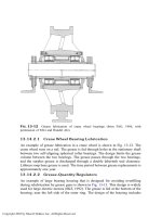
13.3.2 Operating Temperature of the Oil
For selecting an appropriate lubricant, it is important to estimate the operating
temperature of the oil in the bearing. It is possible to estimate the operating oil
temperature by measuring the temperature of the bearing housing. If the machine
is only in design stages, it is possible to estimate the housing temperature by
comparing it to the housing temperature of similar machines. During the
operation of standard bearings that are properly designed, the operating tempera-
ture of the oil is usually in the range of 3

–11

C above that of the bearing
housing. It is relatively simple to measure the housing temperature in an operating
machine and to estimate the oil temperature. Knowledge of the oil temperature is
important for optimal selection of lubricant, oil replacement, and fatigue life
calculations.
Tapered and spherical roller bearings result in higher operating tempera-
tures than do ball bearings or cylindrical roller bearings under similar operating
conditions. The reason is the higher friction coefficient in tapered and spherical
roller bearings.
Copyright 2003 by Marcel Dekker, Inc. All Rights Reserved.
13.3.3 Temperat ure Di¡er ence Between Ri ngs
During operation, the shaft temperature is generally higher than the housing
temperature. The heat is removed from the outer ring through the housing much
faster than from the inner ring through the shaft. There is no good heat transfer

through the small contact area between the rolling elements and rings (theoretical
point or line contact). Therefore, heat from the inner ring is conducted through
the shaft, and heat from the outer ring is conducted through the housing. In
general, heat conduction through the shaft is not as effective as through the
housing. The outer ring and housing have good heat transfer, because they are in
direct contact with the larger body of the machine. In comparison, the inner ring
and shaft have more resistance to heat transfer, because the cross-sectional area of
the shaft is small in comparison to that of the housing as well as to its smaller
surface area, which has lower heat convection relative to the whole machine.
If there is no external source of heat outside the bearing, the operating
temperature of the shaft is always higher than that of the housing. For medium-
speed operation of standard bearings, if the housing is not cooled, the tempera-
tures of the inner ring are in the range of 5

–10

C higher than that of the outer
ring. If the housing is cooled by air flow, the temperature of the inner ring can
increase to 15

–20

C higher than that of the outer ring. An example of air cooling
of the housing is in motor vehicles, where there is air cooling whenever the car is
in motion. It is possible to reduce the temperature difference by means of
adequate oil circulation, which assists in the convection heat transfer between
the rings.
A higher temperature difference can develop in very high-speed bearings.
The temperature difference depends on several factors, such as speed, load, and
type of bearing and shape of the housing. This temperature difference can result

in additional thermal stresses in the bearing.
13.4 ROLLING BEARING LUBRICATION
13.4.1 Objectives of Lubrication
Various types of grease, oils, and, in certain cases, solid lubricants are used for the
lubrication of rolling bearings. Most bearings are lubricated with grease because
it provides effective lubrication and does not require expensive supply systems
(grease can operate with very simple sealing). In most applications, rolling-
element bearings operate successfully with a very thin layer of oil or grease.
However, for high-speed applications, such as turbines, oil lubrication is
important for removing the heat from the bearing or for formation of an EHD
fluid film.
Copyright 2003 by Marcel Dekker, Inc. All Rights Reserved.
The first objective of liquid lubrication is the formation of a thin elasto-
hydrodynamic lubrication film at the rolling contacts between the rolling
elements and the raceways. Under appropriate conditions of load, viscosity, and
bearing speed, this film can completely separate the surfaces of rolling elements
and raceways, resulting in considerable improvement in bearing life.
The second objective of lubrication is to minimize friction and wear in
applications where there is no full EHD film. Experience has indicated that if
proper lubrication is provided, rolling bearings operate successfully for a long
time under mixed lubrication conditions. In practice, ideal conditions of complete
separation are not always maintained. If the height of the surface asperities is
larger than the elastohydrodynamic lubrication film, contact of surface asperities
will take place, and there is a mixed friction (hydrodynamic combined with direct
contact friction).
In addition to pure rolling, there is also a certain amount of sliding contact
between the rolling elements and the raceways as well as between the rolling
elements and the cage. At the sliding surfaces of a rolling bearing, such as the
roller and lip in a roller bearing and at the guiding surface of the cage, a very thin
lubricant film can be formed, resulting in mixed friction under favorable

conditions. Any sliding contact in the bearing requires lubrication to reduce
friction and wear.
The third objective of lubrication (applies to fluid lubricants) is to cool the
bearing and reduce the maximum temperature at the contact of the rolling
elements and the raceways. For effective cooling, sufficient lubricant circulation
should be provided to remove the heat from the bearing. The most effective
cooling is achieved by circulating the oil through an external heat exchanger. But
even without elaborate circulation, a simple oil sump system can enhance the heat
transfer from the bearing by convection. Solid lubricants or greases are not
effective in cooling; therefore, they are restricted to relatively low-speed applica-
tions.
Additional objectives of lubrication are damping of vibrations, corrosion
protection, and removal of dust and wear debris from the raceways via liquid
lubricant. A full EHD fluid film plays an important role as a damper. A full EHD
fluid film acts as noncontact support of the shaft that effectively isolates
vibrations. The fluid film can be helpful in reducing noise and vibrations in a
machine.
Lubricants for rolling bearings include liquid lubricants (mineral and
synthetic oils), greases, and solid lubricants. The most common liquid lubricants
are petroleum-based mineral oils with a long list of additives to improve the
lubrication performance. Also, synthetic lubricants are widely used, such as ester,
polyglycol, and silicone fluoride. Greases are commonly applied in relatively low-
speed applications, where continuous flow for cooling is not essential for
successful operation. The most important advantages of grease are that it seals
Copyright 2003 by Marcel Dekker, Inc. All Rights Reserved.
the bearing from dust and provides effective protection from corrosion. To
minimize maintenance, sealed bearings are widely used, where the bearing is
filled with grease and sealed for the life of the bearing. The grease serves as a
matrix that retains the oil. The oil is slowly released from the grease during
operation.

In addition to grease, oil-saturated solids, such as oil-saturated polymer, are
used successfully for similar applications of sealed bearings. The saturated solid
fills the entire bearing cavity and effectively seals the bearing from contaminants.
The advantage of oil-saturated polymers over grease is that grease can be filled
only into half the bearing internal space in order to avoid churning. In
comparison, oil-saturated solid lubricants are available that can fill the complete
cavity without causing churning. The oil is released from oil-saturated solid
lubricants in a similar way to grease.
Rolling bearings successfully operate in a wide range of environmental
conditions. In certain high-temperature applications, liquid oils or greases cannot
be applied (they oxidize and deteriorate from the heat) and only solid lubricants
can be used. Examples of solid lubricants are PTFE, graphite and molybdenum
disulfide (MoS
2
). Solid lubricants are effective in reducing friction and wear, but
obviously they cannot assist in heat removal as liquid lubricants.
In summary: Lubrication of rolling bearings has several important func-
tions: to form a fluid film, to reduce sliding friction and wear, to transfer heat
away from the bearing, to damp vibrations, and to protect the finished surfaces
from corrosion. Greases and oils are mostly used. Grease packed sealing is
commonly used to protect against the penetration of abrasive particles into the
bearing. Reduction of friction and wear by lubrication is obtained in several ways.
First, a thin fluid film at high pressure can separate the rolling contacts by forming
elastohydrodynamic lubrication. Second, lubrication reduces friction of the
sliding contacts that do not involve rolling, such as between the cage and the
rolling elements or between the rolling elements and the guiding surfaces. Also,
the contacts between the rolling elements and the raceways are not pure rolling,
and there is always a certain amount of sliding. Solid lubricants are also effective
in reducing sliding friction.
13.4.2 Elastohydrodynamic Lubrication

In Chapter 12, the elastohydrodynamic (EHD) lubrication equations were
discussed. EHD theory is concerned with the formation of a thin fluid film at
high pressure at the contact area of a rolling element and a raceway under rolling
conditions. Both the roller and the raceway surfaces are deformed under the load.
In a similar way to fluid film in plain bearings, the oil that is adhering to the
surfaces is drawn into a thin clearance formed between the rolling surfaces. An
important effect is that the viscosity of the oil rises under high pressure; in turn, a
Copyright 2003 by Marcel Dekker, Inc. All Rights Reserved.
load-carrying fluid film is formed at high rolling speed. The clearance thickness,
h
0
, is nearly constant along the fluid film, and it is reducing only near the outlet
side (Fig. 12-20).
Under high loads, the EHD pressure distribution is similar to the pressure
distribution according to the Hertz equations, because the influence of the elastic
deformations dominates the pressure distribution. But at high speeds, the
hydrodynamic effect prevails.
In Chapter 12, the calculation of the film thickness was quite complex. For
many standard applications, engineers often resort to a simplified method based
on charts. The simplified approach also considers the effect of the elastohydro-
dynamic lubrication in improving the fatigue life of the bearing. Even if the EHD
fluid film does not separate completely the rolling surfaces (mixed EHD
lubrication), the lubrication improves the performance, and longer fatigue life
will be obtained. In this chapter, the use of charts is demonstrated for finding the
effect of lubrication in improving the fatigue life of a bearing.
13.4.3 Selection of Liquid Lubricants
The best performance of a rolling bearing is under operating conditions where the
elastohydrodynamic minimum film thickness, h
min
, is thicker than the surface

asperities, R
s
. The required viscosity of the lubricant, m, for this purpose can be
solved for from the EHD equations (see Chapter 12). However, for many standard
applications, designers determine the viscosity by a simpler practical method. It is
based on an empirical chart, where the required viscosity is determined according
to the bearing speed and diameter.
For rolling bearings, the decision concerning the oil viscosity is a
compromise between the requirement of low viscous friction (low viscosity)
and the requirement for adequate EHD film thickness (high viscosity). The
friction of a rolling bearing consists of two components. The first component is
the rolling friction, which results from deformation at the contacts between a
rolling element and a raceway. The second friction component is viscous
resistance of the lubricant to the motion of the rolling elements. The first
component of rolling friction is a function of the elastic modulus, geometry,
and bearing load. The second component of viscous friction increases with
lubricant viscosity, quantity of oil in the bearing, and bearing speed. The viscous
component increases with speed, so it becomes a dominant factor in high–speed
machinery.
It is possible to minimize the viscous resistance by applying a very small
quantity of oil, just sufficient to form a thin layer over the contact surface. In
addition, using low-viscosity oil can reduce the viscous resistance. However,
minimum lubricant viscosity must be maintained to ensure elastohydrodynamic
lubrication with adequate fluid film thickness.
Copyright 2003 by Marcel Dekker, Inc. All Rights Reserved.
For lubricant selection, a knowledge of the operating bearing temperature is
required. One must keep in mind that the lubricant viscosity decreases with
temperature. In applications where the bearing temperature is expected to rise
significantly, lubricant of higher initial viscosity should be selected. It is possible
to reduce the bearing operating temperature via oil circulation for removing the

heat and cooling the bearing. The final bearing temperature rise, above the
ambient temperature, is affected by many factors, such as speed and load. A
simplified method for estimating the bearing temperature was discussed earlier.
For predicting the operating temperature, this method relies mostly on experience
with similar machinery for determining the heat transfer coefficients.
For bearings that do not dissipate heat from outside the bearing and that
operate at moderate speeds and under average loads, it is possible to estimate the
oil temperature by measuring the housing temperature. During operation, the
temperature of the oil is usually in the range of 3

–11

C above that of the bearing
housing. This simple temperature estimation is widely used for lubricant selec-
tion.
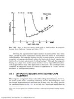
In order to simplify the selection of oil viscosity, charts based on bearing
speed and bearing average diameter are used. Figure 13-1 is used for determining
the minimum oil viscosity for lubrication of rolling-element bearings as a
function of bearing size and speed.
The ordinate on the left side shows the kinematic viscosity in metric units,
mm
2
=s ðcStÞ. The ordinate on the right side shows the viscosity in Saybolt
universal seconds (SUS). The abscissa is the pitch diameter, d
m
, in mm, which is
the average of internal bore, d, and outside bearing diameter, D.
d
m
¼

d þ D
2
ð13-17Þ
The diagonal straight lines in Fig. 13-1 are for the various bearing speed N in
RPM (revolutions per minute). The dotted lines show examples of determining
the required lubricant viscosity.
Example Problem 13-1
Calculation of Minimum Viscosity
A rolling bearing has a bore diameter d ¼ 45 mm and an outside diameter
D ¼ 85 mm. The bearing rotates at 2000 RPM. Find the required minimum
viscosity of the lubricant.
Copyright 2003 by Marcel Dekker, Inc. All Rights Reserved.