Bearing Design in Machinery Episode 1 Part 9 pps

The preceding equation is converted into dimensionless terms (see Example
Problem 6-1):
"
xx ¼
x
ffiffiffiffiffiffiffiffiffiffi
2Rh
n
p
;
"
hh ¼
h
h
n
; and h
0
¼
h
0
h
n
dp
dx
¼
6mUð1 þxÞ
h
2
n
"
xx

2
À
"
xx
2
0
ð1 þ
"
xx
2
Þ
3
Converting the pressure gradient to dimensionless form yields
h
2
n
ffiffiffiffiffiffiffiffiffiffi
2Rh
n
p
6mU
dp ¼ð1 þ xÞ
"
xx
2
À
"
xx
2
0

ð1 þ
"
xx
2
Þ
3
d
"
xx
The left hand side of the equation is the dimensionless pressure:
"
pp ¼ð1 þ xÞ
h
2
n
ffiffiffiffiffiffiffiffiffiffiffi
2RH
n
p
1
6mU
ð
p
0
dp ¼ð1 þ xÞ
ð
x
À1
"
xx

2
À
"
xx
2
0
ð1 þ
"
xx
2
Þ
3
d
"
xx þ p
0
Here, p
0
is a constant of integration, which is atmospheric pressure far from the
minimum clearance. In this equation, p
0
and x
0
are two unknowns that can be
solved for by the practical boundary conditions of the pressure wave; compare to
Eqs. (6-67):
p ¼ p
0
at x ¼ x
1

dp
dx
¼ 0atx ¼ x
2
p ¼ 0atx ¼ x
2
Atmospheric pressure is zero, and the first boundary condition results in
p
0
¼ 0. The location of the end of the pressure wave, x
2
, is solved by iterations.
The solution is performed by guessing a value for x ¼ x
2
; then x
0
is taken as x
2
,
because at that point the pressure gradient is zero.
The solution requires iterations in order to find x
0
¼ x
2
, which satisfies the
boundary conditions. For each iteration, integration is performed in the bound-
aries from 0 to x
2
, and the solution is obtained when the pressure at x
2

is very
close to zero.
For numerical integration, the boundary
"
xx
1
, where the pressure is zero, is
taken as a small value, such as
"
xx
1
¼À4. The solution is presented in Fig. 6-10.
The curves indicate that the pressure wave is higher for higher rolling ratios. This
means that the rolling plays a stronger role in hydrodynamic pressure generation
in comparison to sliding.
Copyright 2003 by Marcel Dekker, Inc. All Rights Reserved.
6-2 A flat plate slides on a lubricated cylinder as shown in Fig. 4-7. The
cylinder radius is R, the lubricant viscosity is m, and the minimum
clearance between the stationary cylinder and plate is h
n
. The elastic
deformation of the cylinder and plate is negligible.
1. Apply numerical iterations, and plot the dimensionless
pressure wave. Assume practical boundary conditions of
the pressure, according to Eq. 6.67.
2. Find the expression for the load capacity by numerical
integration.
6-3 In problem 6-2, the cylinder diameter is 250 mm, the plate slides at
U ¼ 0:5m=s, and the minimum clearance is 1 mm (0.001 mm). The
lubricant viscosity is constant, m ¼ 10

À4
N-s=m
2
. Find the hydro-
dynamic load capacity.
6-4 Oil is fed into a journal bearing by a pump. The supply pressure is
sufficiently high to avoid cavitation. The bearing operates at an
eccentricity ratio of e ¼ 0:85, and the shaft speed is 60 RPM. The
bearing length is L ¼ 3D, the journal diameter is D ¼ 80 mm, and
the clearance ratio is C=R ¼ 0:002. Assume that the pressure is
constant along the bearing axis and there is no axial flow (long-
bearing theory).
a. Find the maximum load capacity for a lubricant SAE 20
operating at an average fluid film temperature of 60

C.
b. Find the bearing angle y where there is a peak pressure.
c. What is the minimum supply pressure from the pump in
order to avoid cavitation and to have only positive pressure
around the bearing?
6-5 An air bearing operates inside a pressure vessel that has sufficiently
high pressure to avoid cavitation in the bearing. The average viscosity
of the air inside the bearing is m ¼ 2 Â 10
À4
N-s=m
2
. The bearing
operates at an eccentricity ratio of e ¼ 0:85. The bearing length is
L ¼ 2D, the journal diameter is D ¼ 30 mm, and the clearance ratio
is C=R ¼ 8 Â 10

À4
. Assume that the pressure is constant along the
bearing axis and there is no axial flow (long-bearing theory).
a. Find the journal speed in RPM that is required for a bearing
load capacity of 200 N. Find the bearing angle y where
there is a peak pressure.
b. What is the minimum ambient pressure around the bearing
(inside the pressure vessel) in order to avoid cavitation and
to have only positive pressure around the bearing?
Copyright 2003 by Marcel Dekker, Inc. All Rights Reserved.
7
Short Journal Bearings
7.1 INTRODUCTION
The term short journal bearing refers to a bearing of a short length, L,in
comparison to the diameter, D, ðL ( DÞ. The bearing geometry and coordinates
are shown in Fig. 7-1. Short bearings are widely used and perform successfully in
various machines, particularly in automotive engines. Although the load capacity,
per unit length, of a short bearing is lower than that of a long bearing, it has the
following important advantages.
1. In comparison to a long bearing, a short bearing exhibits improved heat
transfer, due to faster oil circulation through the bearing clearance. The
flow rate of lubricant in the axial direction through the bearing
clearance of a short bearing is much faster than that of a long bearing.
This relatively high flow rate improves the cooling by continually
replacing the lubricant that is heated by viscous shear. Overheating is a
major cause for bearing failure; therefore, operating temperature is a
very important consideration in bearing design.
2. A short bearing is less sensitive to misalignment errors. It is obvious
that short bearings reduce the risk of damage to the journal and the
bearing edge resulting from misalignment of journal and bearing bore

centrelines.
3. Wear is reduced, because abrasive wear particles and dust are washed
away by the oil more easily in short bearings.
Copyright 2003 by Marcel Dekker, Inc. All Rights Reserved.
use the short-bearing equation to calculate finite-length bearings, the bearing
design will be on the safe side, with high safety coefficient. For this reason, the
short-journal equations are widely used by engineers for the design of hydro-
dynamic journal bearings, even for bearings that are not very short, if there is no
justification to spend too much time on elaborate calculations to optimize the
bearing design.
7.2 SHORT-BEARING ANALYSIS
The starting point of the derivation is the Reynolds equation, which was
discussed in Chapter 5. Let us recall that the Reynolds equation for incompres-
sible Newtonian fluids is
@
@x
h
3
m
@p
@x

þ
@
@z
h
3
m
@p
@z


¼ 6ðU
1
À U
2
Þ
@h
@x
þ 12ðV
2
À V
1
Þð7-2Þ
Based on the assumption that the pressure gradient in the x direction can be
disregarded, we have
@
@x
h
3
m
@p
@x

% 0 ð7-3Þ
Thus, the Reynolds equation (7-2) reduces to the following simplified form:
@
@z
h
3
m

@p
@z

¼ 6ðU
1
À U
2
Þ
@h
@x
þ 12ðV
2
À V
1
Þð7-4Þ
In a journal bearing, the surface velocity of the journal is not parallel to the x
direction along the bore surface, and it has a normal component V
2
(see diagram
of velocity components in Fig. 6-2). The surface velocity components of the
journal surface are
U
2
% U; V
2
% U
@h
@x
ð7-5Þ
On the stationary sleeve, the surface velocity components are zero:

U
1
¼ 0; V
1
¼ 0 ð7-6Þ
After substituting Eqs. (7-5) and (7-6) into the right-hand side of Eq. (7-4), it
becomes
6ðU
1
À U
2
Þ
@h
@x
þ 12ðV
2
À V
1
Þ¼6ð0 ÀUÞ
@h
@x
þ 12U
@h
@x
¼ 6U
@h
@x
ð7-7Þ
Copyright 2003 by Marcel Dekker, Inc. All Rights Reserved.
FIG. 7-2 Pressure wave at z ¼ 0 in a short bearing for various values of e.

Copyright 2003 by Marcel Dekker, Inc. All Rights Reserved.
The Reynolds equation for a short journal bearing is finally simplified to the form
@
@z
h
3
m
@p
@z

¼ 6U
@h
@x
ð7-8Þ
The film thickness h is solely a function of x and is constant for the purpose of
integration in the z direction. Double integration results in the following parabolic
pressure distribution, in the z direction, with two constants, which can be obtained
from the boundary conditions of the pressure wave:
p ¼À
6mU
h
3
dh
dx
z
2
2
þ C
1
z þ C

2
ð7-9Þ
At the two ends of the bearing, the pressure is equal to the atmospheric pressure,
p ¼ 0. These boundary conditions can be written as
p ¼ 0atz ¼Æ
L
2
ð7-10Þ
Solving for the integration constants, and substituting the function for h in a
journal bearing, hðyÞ¼Cð1 þe cos y), the following expression for the pressure
distribution in a short bearing (a function of y and z) is obtained:
pðy; zÞ¼
3mU
RC
2
L
2
4
À z
2

e sin y
ð1 þe cosÞ
3
ð7-11Þ
In a short journal bearing, the film thickness h is converging (decreasing h
vs. y) in the region ð0 < y < pÞ, resulting in a viscous wedge and a positive
pressure wave. At the same time, in the region ðp < y < 2pÞ, the film thickness h
is diverging (increasing h vs. y ). In the diverging region ðp < y < 2pÞ, Eq. (7-11)
predicts a negative pressure wave (because sin y is negative). The pressure

according to Eq. (7-11) is an antisymmetrical function on the two sides of y ¼ p.
In an actual bearing, in the region of negative pressure ðp < y < 2pÞ, there
is fluid cavitation and the fluid continuity is breaking down. There is fluid
cavitation whenever the negative pressure is lower than the vapor pressure.
Therefore, Eq. (7-11) is no longer valid in the diverging region. In practice, the
contribution of the negative pressure to the load capacity can be disregarded.
Therefore in a short bearing, only the converging region with positive pressure
ð0 < y < pÞ is considered for the load capacity of the oil film (see Fig. 7-2).
Similar to a long bearing, the load capacity is solved by integration of the
pressure wave around the bearing. But in the case of a short bearing, the pressure
is a function of z and y. The following are the two equations for the integration
Copyright 2003 by Marcel Dekker, Inc. All Rights Reserved.
for the load capacity components in the directions of W
x
and W
y
of the bearing
centerline and the normal to it:
W
x
¼À2
ð
p
0
ð
L=2
0
p cos y Rdy dz ¼À
mUL
3

2C
2
ð
p
0
e sin y cos y
ð1 þ e cos yÞ
3
dy ð7-12aÞ
W
y
¼ 2
ð
p
0
ð
L=2
0
p sin y dy dz ¼
mUL
3
2C
2
ð
p
0
e sin
2
y
ð1 þe cos yÞ

3
dy ð7-12bÞ
The following list of integrals is useful for short journal bearings.
J
11
¼
ð
p
0
sin
2
y
ð1 þ e cos yÞ
3
dy ¼
p
2ð1 Àe
2
Þ
3=2
ð7-13aÞ
J
12
¼
ð
p
0
sin ycos y
ð1 þ e cos yÞ
3

dy ¼
À2e
ð1 Àe
2
Þ
2
ð7-13bÞ
J
22
¼
ð
p
0
cos
2
y
ð1 þ e cos yÞ
3
dy ¼
pð1 þ2e
2
Þ
2ð1 Àe
2
Þ
5=2
ð7-13cÞ
The load capacity components are functions of the preceding integrals:
W
x

¼À
mUL
3
2C
2
e J
12
ð7-14Þ
W
y
¼
mUL
3
2C
2
e J
11
ð7-15Þ
Using Eqs. (7-13) and substitution of the values of the integrals results in the
following expressions for the two load components:
W
x
¼
mUL
3
C
2
e
2
ð1 Àe

2
Þ
2
ð7-16aÞ
W
y
¼
mUL
3
4C
2
pe
ð1 Àe
2
Þ
3=2
ð7-16bÞ
Equations (7-16) for the two load components yield the resultant load capacity of
the bearing, W :
W ¼
mUL
3
4C
2
e
ð1 Àe
2
Þ
2
½p

2
ð1 Àe
2
Þþ16e
2

1=2
ð7-17Þ
The attitude angle, f, is determined from the two load components:
tan f ¼
W
y
W
x
ð7-18Þ
Copyright 2003 by Marcel Dekker, Inc. All Rights Reserved.
Via substitution of the values of the load capacity components, the expression for
the attitude angle of a short bearing becomes
tan f ¼
p
4
ð1 Àe
2
Þ
1=2
e
ð7-19Þ
7.3 FLOW IN THE AXIAL DIRECTION
The velocity distribution of the fluid in the axial, z, direction is
w ¼ 3U

zh
0
Rh
3
ðy
2
À hyÞð7-20Þ
Here,
h
0
¼
dh
dx
ð7-21Þ
The gradient h
0
is the clearance slope (wedge angle), which is equal to the fluid
film thickness slope in the direction of x ¼ Ry (around the bearing). This gradient
must be negative in order to result in a positive pressure wave as well as positive
flow, w, in the z direction.
Positive axial flow is directed outside the bearing (outlet flow from the
bearing). There is positive axial flow where h is converging (decreasing h vs. x)in
the region ð0 < y < pÞ. At the same time, there is inlet flow, directed from
outside into the bearing, where h is diverging (increasing h vs. y) in the region
ðp < y < 2pÞ. In the diverging region, h
0
> 0, there is fluid cavitation that is
causing deviation from the theoretical axial flow predicted in Eq. (7-20).
However, in principle, the lubricant enters into the bearing in the diverging
region and leaves the bearing in the converging region. In a short bearing, there is

much faster lubricant circulation relative to that in a long bearing. Fast lubricant
circulation reduces the peak temperature of the lubricant. This is a significant
advantage of the short bearing, because high peak temperature can cause bearing
failure.
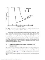
7.4 SOMMERFELD NUMBER OF A SHORT
BEARING
The definition of the dimensionless Sommerfeld number for a short bearing is
identical to that for a long bearing; however, for a short journal bearing, the
expression of the Sommerfeld number is given as,
S ¼
mn
P
R
C

2
¼
D
L

2
ð1 Àe
2
Þ
2
pe½p
2
ð1 Àe
2
Þþ16e

2

1=2
ð7-22Þ
Copyright 2003 by Marcel Dekker, Inc. All Rights Reserved.
Let us recall that the Sommerfeld number of a long bearing is only a function of
e. However, for a short bearing, the Sommerfeld number is a function of e as well
as the ratio L=D.
7.5 VISCOUS FRICTION
The friction force around a bearing is obtained by integration of the shear
stresses. The shear stress in a short bearing is
t ¼ m
U
h
ð7-23Þ
For the purpose of computing the friction force, the shear stresses are integrated
around the complete bearing. The fluid is present in the diverging region
(p < y < 2p), and it is contributing to the viscous friction, although its contribu-
tion to the load capacity has been neglected. The friction force, F
f
, is obtained by
integration of the shear stress, t, over the complete surface area of the journal:
F
f
¼
ð
ðAÞ
t dA ð7-24Þ
Substituting dA ¼ LR dy, the friction force becomes
F

f
¼ RL
ð
2p
0
t dy ð7-25Þ
To solve for the friction force, we substitute the expression for h into Eq. (7-23)
and substitute the resulting equation of t into Eq. (7-25). For solving the integral,
the following integral equation is useful:
J
1
¼
ð
2p
0
1
1 þ cos y
dy ¼
2p
ð1 Àe
2
Þ
1=2
ð7-26Þ
Note that J
1
has the limits of integration 0 2p, while for the first three integrals
in Eqs. (7-13), the limits are 0
p. The final expression for the friction force is
F

f
¼
mLRU
C
ð
2p
0
dy
1 þ e cos y
¼
mLRU
C
2p
ð1 Àe
2
Þ
1=2
ð7-27Þ
The bearing friction coefficient f is defined as
f ¼
F
f
W
ð7-28Þ
The friction torque T
f
is
T
f
¼ F

f
R; T
f
¼
mLR
2
U
C
2p
ð1 Àe
2
Þ
1=2
ð7-29Þ
Copyright 2003 by Marcel Dekker, Inc. All Rights Reserved.
The energy loss per unit of time,
_
EE
f
is determined by the following:
_
EE
f
¼ F
f
U ð7-30aÞ
Substituting Eq. (7-27) into Eq. (7-30a) yields the following expression for the
power loss on viscous friction:
_
EE

f
¼
mLRU
2
C
2p
ð1 Àe
2
Þ
1=2
ð7-30bÞ
7.6 JOURNAL BEARING STIFFNESS
Journal bearing stiffness, k, is the rate of increase of load W with displacement e
in the same direction, dW=de (similar to that of a spring constant). High stiffness
is particularly important in machine tools, where any displacement of the spindle
centerline during machining would result in machining errors. Hydrodynamic
journal bearings have low stiffness at low eccentricity (under light load).
The displacement of a hydrodynamic bearing is not in the same direction as
the force W . In such cases, the journal bearing has cross-stiffness components.
The stiffness components are presented as four components related to the force
components W
x
and W
y
and the displacement components in these directions.
In a journal bearing, the load is divided into two components, W
x
and W
y
,

and the displacement of the bearing center, e, is divided into two components, e
x
and e
y
. The two components of the journal bearing stiffness are
k
x
¼
dW
x
de
x
; k
y
¼
dW
y
de
y
ð7-31Þ
and the two components of the cross-stiffness are defined as
k
xy
¼
dW
x
de
y
; k
y

¼
dW
y
de
x
ð7-32Þ
Cross-stiffness components cause instability, in the form of an oil whirl in journal
bearings.
Example Problem 7-1
A short bearing is designed to operate with an eccentricity ratio e ¼ 0:8. The
journal diameter is 60 mm, and its speed is 1500 RPM. The journal is supported
by a short hydrodynamic bearing of length L=D ¼ 0:5, and clearance ratio
C=R ¼ 10
À3
. The radial load on the bearing is 1 metric ton (1 metric
ton ¼ 9800 [N]).
a. Assume that infinitely-short-bearing theory applies to this bearing, and
find the Sommerfeld number.
Copyright 2003 by Marcel Dekker, Inc. All Rights Reserved.
b. Find the minimum viscosity of the lubricant for operating at e ¼ 0:8.
c. Select a lubricant if the average bearing operating temperature is 80

C.
Solution
a. Sommerfeld Number
The Sommerfeld number is
S ¼
mn
P
R

C

2
¼
D
L

2
ð1 Àe
2
Þ
2
pe½p
2
ð1 Àe
2
Þþ16e
2

1=2
From the right-hand side of the equation,
S ¼ð2Þ
2
ð1 À 0:8
2
Þ
2
p0:8½p
2
ð1 À0:8

2
Þþ16 Â 0:8
2

1=2
¼
0:36
2
p  0:8  3:71
¼ 0:0139
b. Minimum Viscosity
The average pressure is
P ¼
W
LD
¼
9800
0:06 Â0:03
¼ 5:44 Â 10
6
Pa
The load in SI units (newtons) is 9800 [N], and the speed is n ¼
1500=60 ¼ 25 RPS.
The viscosity is determined by equating:
S ¼
mn
P
R
C


2
¼ 0:0139
m ¼
5:44 Â 10
6
 0:0139
25 Â 10
6
¼ 0:0030 ½N-s=m
2

c. Lubricant
For lubricant operating temperature of 80

C, mineral oil SAE 10 has suitable
viscosity of 0.003 [N-s=m
2
] (Fig. 2-3). This is the minimum required viscosity for
the operation of this bearing with an eccentricity ratio no higher than e ¼ 0:8.
Example Problem 7-2
A journal of 75-mm diameter rotates at 3800 RPM. The journal is supported by a
short hydrodynamic bearing of length L ¼ D=4 and a clearance ratio
C=R ¼ 10
À3
. The radial load on the bearing is 0.5 metric ton, (1 metric
ton ¼ 9800 [N]). The lubricant is SAE 40, and the operating temperature of
the lubricant in the bearing is 80

C.
Copyright 2003 by Marcel Dekker, Inc. All Rights Reserved.

a. Assume infinitely-short-bearing theory, and find the eccentricity ratio,
e, of the bearing (use a graphic method to solve for e) and the minimum
film thickness, h
n
.
b. Derive the equation for the pressure wave around the bearing, at the
center of the width (at z ¼ 0).
c. Find the hydrodynamic friction torque and the friction power losses (in
watts).
Solution
The following conversion is required for calculation in SI units:
Speed of shaft: n ¼ 3800= 60 ¼ 63:3 [RPS]
Radial load: W ¼ 0:5 Â 9800 ¼ 4900 [N]
Axial length of shaft: L ¼ D=4 ¼ 0:075=4 ¼ 0:01875 [m]
C=R ¼ 10
À3
; hence R=C ¼ 10
3
.
a. Eccentricity Ratio and Minimum Film Thickness
For an operating temperature of T ¼ 80

C, the viscosity of SAE-40 oil is
obtained from the viscosity–temperature chart: m ¼ 0:0185 ½N-s=m
2
. The equa-
tion for the load capacity is applied to solve for the eccentricity ratio, e, the only
unknown in the following equation:
W ¼
mUL

3
4C
2
e
ð1 Àe
2
Þ
2
½p
2
ð1 Àe
2
Þþ16e
2

1=2
ð7-32Þ
To simplify the mathematical derivation of e, the following substitution is helpful:
f ðeÞ¼
e
ð1 À e
2
Þ
2
½p
2
ð1 Àe
2
Þþ16e
2


1=2
ð7-33Þ
First, we can solve for f ðeÞ, and later we can obtain the value of e from the graph
of f ðeÞ vs. e (Fig. 7-3).
Equations (7-32) and (7-33) yield
f ðeÞ¼
4WC
2
mUL
3
¼
4W ð10
À3
 D=2Þ
2
mpnDðD=4Þ
3
¼
4 Â 16 Â 4900 Â 10
À6
0:0185p  63:3ð0:075Þ
2
¼ 15:15
According to the curve of f ðeÞ vs. e, for f ðeÞ¼15:15, the eccentricity of the
bearing is e ¼ 0:75.
Copyright 2003 by Marcel Dekker, Inc. All Rights Reserved.
The pressure wave at the width center, z ¼ 0, is
pðyÞ¼
3mUL

2
4h
3
Ce sin y
R
pðyÞðat z ¼ 0Þ¼
3  0:0185  p  63:3 Â0:075 Â0:075
2
 0:75
64 Â 10
3
Â
sin y
ð1 þ0:75 cos yÞ
3
pðyÞðat z ¼ 0Þ¼
5:5 Â 10
À8
sin y
ð1 þ 0:75 cos yÞ
3
c. Friction Torque and Friction Power Loss
We find the friction torque as follows:
T
f
¼ F
f
R ¼
mLR
2

U
C
2p
ð1 Àe
2
Þ
1=2
¼
0:0185 Â0:01875 Âð0: 075=2ÞÂp  0:075 Â63:3
10
À3
2p
ð1 À0:75
2
Þ
1=2
T
f
¼ 1:80 N-m
The friction power loss is found as follows:
_
EE
f
¼ T
f
o
_
EE
f
¼

mLRU
2
C
2p
ð1 Àe
2
Þ
1=2
_
EE
f
¼
0:0185 Â0:01875 Âðp  63:3 Â0:075Þ
2
10
À3
2p
ð1 À 0:75
2
Þ
1=2
¼ 733 ½W
Problems
7-1 A short bearing is designed to operate with an eccentricity ratio of
e ¼ 0:7. Find the journal diameter if the speed is 30,000 RPM and the
radial load on the bearing is 8000 N. The bearing length ratio
L=D ¼ 0:6, and the clearance ratio is C=R ¼ 10
À3
. The lubricant is
SAE 30 and the average operating temperature in the bearing is 70


C.
Assume that infinitely-short-bearing theory applies.
7-2 Plot the dimensionless pressure distribution (function of y) at the
bearing center, z ¼ 0, in Example Problem 7-2.
7-3 A short bearing is designed to operate with an eccentricity ratio of
e ¼ 0:75. The journal is 80 mm in diameter, and its speed is
Copyright 2003 by Marcel Dekker, Inc. All Rights Reserved.
3500 RPM. The journal is supported by a short hydrodynamic
bearing of length D=L ¼ 4 and a clearance ratio of C=R ¼ 10
À3
.
The radial load on the bearing is 1000 N.
a. Assume that infinitely-short-bearing theory applies to this
bearing, and find the minimum viscosity of the lubricant.
b. Select a lubricant for an average operating temperature in
the bearing of 60

C.
7-4 The journal speed of a 100 mm diameter journal is 2500 RPM. The
journal is supported by a short hydrodynamic bearing of length
L ¼ 0:6D and a clearance ratio of C=R ¼ 10
À3
. The radial load on
the bearing is 10,000 [N]. The lubricant is SAE 30, and the operating
temperature of the lubricant in the bearing is 70

C.
a. Assume infinitely-short-bearing theory, and find the eccen-
tricity ratio, e, of the bearing and the minimum film

thickness, h
n
(use a graphic method to solve for e).
b. Derive the equation and plot the pressure distribution
around the bearing, at the center of the width (at z ¼ 0).
c. Find the hydrodynamic friction torque and the friction
power losses (in watts) for each bearing.
Copyright 2003 by Marcel Dekker, Inc. All Rights Reserved.
8
Design Charts for Finite-Length
Journal Bearings
8.1 INTRODUCTION
In the preceding chapters, the analysis of infinitely long and short journal
bearings have been presented. In comparison, the solution of a finite-length
journal bearing (e.g., L=D ¼ 1) is more complex and requires a computer
program for a numerical solution of the Reynolds equation. The first numerical
solution of the Reynolds equation for a finite-length bearing was performed by
Raimondi and Boyd (1958). The results were presented in the form of dimen-
sionless charts and tables, which are required for journal bearing design. The
presentation of the results in the form of dimensionless charts and tables is
convenient for design purposes because one does not need to repeat the numerical
solution for each bearing design. The charts and tables present various dimen-
sionless performance parameters, such as minimum film thickness, friction, and
temperature rise of the lubricant as a function of the Sommerfeld number, S. Let
us recall that the dimensionless Sommerfeld number is defined as
S ¼
R
C

2

mn
P
ð8-1Þ
Copyright 2003 by Marcel Dekker, Inc. All Rights Reserved.
where n is the speed of the journal in revolutions per second (RPS), R is the
journal radius, C is the radial clearance, and P is the average bearing pressure
(load, F, per unit of projected contact area of journal and bearing), given by
P ¼
F
2RL
¼
F
DL
ð8-2Þ
Note that S is a dimensionless number, and any system of units can be applied for
its calculation as long as one is consistent with the units. For instance, if the
Imperial unit system is applied, length should be in inches, force in lbf, and m in
reynolds [lbf-s=in.
2
]. In SI units, length is in meters, force in newtons, and the
viscosity, m, in [N-s=m
2
]. The journal speed, n, should always be in revolutions
per second (RPS), irrespective of the system of units used, and the viscosity, m,
must always include seconds as the unit of time.
8.2 DESIGN PROCEDURE
The design procedure starts with the selection of the bearing dimensions: the
journal diameter D, the bearing length L, and the radial clearance between the
bearing and the journal C. At this stage of the design, the shaft diameter should
already have been computed according to strength-of-materials considerations.

However, in certain cases the designer may decide, after preliminary calculations,
to increase the journal diameter in order to improve the bearing hydrodynamic
load capacity.
One important design decision is the selection of the L=D ratio. It is
obvious from hydrodynamic theory of lubrication that a long bearing has a higher
load capacity (per unit of length) in comparison to a shorter bearing. On the other
hand, a long bearing increases the risk of bearing failure due to misalignment
errors. In addition, a long bearing reduces the amount of oil circulating in the
bearing, resulting in a higher peak temperature inside the lubrication film and the
bearing surface. Therefore, short bearings (L=D ratios between 0.5 and 0.7) are
recommended in many cases. Of course, there are many unique circumstances
where different ratios are selected.
The bearing clearance, C, is also an important design factor, because the
load capacity in a long bearing is proportional to ðR=CÞ
2
. Experience over the
years has resulted in an empirical rule used by most designers. They commonly
select a ratio R=C of about 1000. The ratio R=C is equal to the ratio D=DD
between the diameter and the diameter clearance; i.e., a journal of 50-mm
diameter should have a 50-mm (fifty-thousandth of a millimeter)-diameter
clearance. The designer should keep in mind that there are manufacturing
tolerances of bearing bore and journal diameters, resulting in significant toler-
ances in the journal bearing clearance, DD. The clearance can be somewhat
smaller or larger, and thus the bearing should be designed for the worst possible
Copyright 2003 by Marcel Dekker, Inc. All Rights Reserved.
scenario. In general, high-precision manufacturing is required for journal bear-
ings, to minimize the clearance tolerances as well as to achieve good surface
finish and optimal alignment.
For bearings subjected to high dynamic impacts, or very high speeds,
somewhat larger bearing clearances are chosen. The following is an empirical

equation that is recommended for high-speed journal bearings having an L=D
ratio of about 0.6:
C
D
¼ð0:0009 þ
n
83;000
Þð8-3Þ
where n is the journal speed (RPS). This equation is widely used to determine the
radial clearance in motor vehicle engines.
8.3 MINIMUM FILM THICKNESS
One of the most critical design decisions concerns the minimum film thickness,
h
n
. Of course, the minimum fluid film thickness must be much higher than the
surface roughness, particularly in the presence of vibrations. Even for statically
loaded bearings, there are always unexpected disturbances and dynamic loads,
due to vibrations in the machine, and a higher value of the minimum film
thickness, h
n
, is required to prevent bearing wear. In critical applications, where
the replacement of bearings is not easy, such as bearings located inside an engine,
more care is required to ensure that the minimum film thickness will never be
reduced below a critical value at which wear can initiate.
Another consideration is the fluid film temperature, which can increase
under unexpected conditions, such as disturbances in the operation of the
machine. The temperature rise reduces the lubricant viscosity; in turn, the oil
film thickness is reduced. For this reason, designers are very careful to select h
n
much larger than the surface roughness. The common design practice for

hydrodynamic bearings is to select a minimum film thickness in the range of
10–100 times the average surface finish (in RMS). For instance, if the journal and
the bearing are both machined by fine turning, having a surface finish specified by
an RMS value of 0.5 mm (0.5 thousandths of a millimeter), the minimum film
thickness can be within the limits of 5–50 mm. High h
n
values are chosen in the
presence of high dynamic disturbances, whereas low values of h
n
are chosen for
steady operation that involves minimal vibrations and disturbances.
Moreover, if it is expected that dust particles would contaminate the
lubricant, a higher minimum film thickness, h
n
, should be selected. Also, for
critical applications, where there are safety considerations, or where bearing
failure can result in expensive machine downtime, a coefficient of safety is
applied in the form of higher values of h
n
.
Copyright 2003 by Marcel Dekker, Inc. All Rights Reserved.