Bearing Design in Machinery Episode 1 Part 7 pps

However, if the x coordinate is in the direction of a diverging clearance (the
clearance increases with x), as shown in Fig. (1-2), Eq. (5-15) changes its sign
and takes the following form:
dp
dx
¼ 6Um
h
0
À h
h
3
for initial
@h
@x
> 0 ðpositive slope in Fig: 4-5Þ
ð5-15Þ
5.4 FLUID FILM BETWEEN A FLAT PLATE AND A
CYLINDER
A fluid film between a plate and a cylinder is shown in Fig. 5-4. In Chapter 4, the
pressure wave for relative sliding is derived, where the cylinder is stationary and a
flat plate has a constant velocity in the x direction. In the following example, the
previous problem is extended to a combination of rolling and sliding. In this case,
the flat plate has a velocity U in the x direction and the cylinder rotates at an
angular velocity o around its stationary center. The coordinate system (x, y)is
stationary.
In Sec. 4.8, it is mentioned that there is a significant pressure wave only in
the region close to the minimum film thickness. In this region, the slope between
the two surfaces (the fluid film boundaries), as well as between the two surface
velocities, is of a very small angle a. For a small a, we can approximate that
cos a % 1.
FIG. 5-4 Fluid film between a moving plate and a rotating cylinder.

Copyright 2003 by Marcel Dekker, Inc. All Rights Reserved.
In Fig. 5-4, the surface velocity of the cylinder is not parallel to the x
direction and it has a normal component V
2
. The surface velocities on the rotating
cylinder surface are
U
2
¼ oR cos a % oRV
2
% oR
@h
@x
ð5-16Þ
At the same time, on the lower plate there is only velocity U in the x direction and
the boundary velocity is
U
1
¼ UV
1
¼ 0 ð5-17Þ
Substituting Eqs. (5-16) and (5-17) into the right side of Eq. (5-11), yields
6ðU
1
À U
2
Þ
@h
@x
þ 12ðV

2
À V
1
Þ¼6ðU À o RÞ
@h
@x
þ 12oR
@h
@x
¼ 6ðU þ oRÞ
@h
@x
ð5-18Þ
The Reynolds equation for a fluid film between a plate and a cylinder becomes
@
@x
h
3
m
@p
@x

þ
@
@z
h
3
m
@p
@z


¼ 6ðU þ oRÞ
@h
@x
ð5-19Þ
For a long bearing, the pressure gradient in the axial direction is negligible,
@p=@z ffi 0. Integration of Eq. (5-19) yields
dp
dx
¼ 6mðU þ oRÞ
h À h
0
h
3
ð5-20Þ
This result indicates that the pressure gradient, the pressure wave, and the load
capacity are proportional to the sum of the two surface velocities in the x
direction. The sum of the plate and cylinder velocities is ðU þ oRÞ. In the case of
pure rolling, U ¼ oR, the pressure wave, and the load capacity are twice the
magnitude of that generated by pure sliding. Pure sliding is when the cylinder is
stationary, o ¼ 0, and only the plate has a sliding velocity U.
The unknown constant h
0
, (constant of integration) is the film thickness at
the point of a peak pressure, and it can be solved from the boundary conditions of
the pressure wave.
5.5 TRANSITION TO TURBULENCE
For the estimation of the Reynolds number, Re, the average radial clearance, C,is
taken as the average film thickness. The Reynolds number for the flow inside the
clearance of a hydrodynamic journal bearing is

Re ¼
UrC
m
¼
UC
n
ð5-21Þ
Copyright 2003 by Marcel Dekker, Inc. All Rights Reserved.
Here, U is the journal surface velocity, as shown in Fig. 1-2 and n is the kinematic
viscosity n ¼ m=r. In most cases, hydrodynamic lubrication flow involves low
Reynolds numbers. There are other examples of thin-film flow in fluid mechanics,
such as the boundary layer, where Re is low.
The flow in hydrodynamic lubrication is laminar at low Reynolds numbers.
Experiments in journal bearings indicate that the transition from laminar to
turbulent flow occurs between Re ¼ 1000 and Re ¼ 1600. The value of the
Reynolds number at the transition to turbulence is not the same in all cases. It
depends on the surface finish of the rotating surfaces as well as the level of
vibrations in the bearing. The transition is gradual: Turbulence starts to develop at
about Re ¼ 1000; and near Re ¼ 1600, full turbulent behavior is maintained. In
hydrodynamic bearings, turbulent flow is undesirable because it increases the
friction losses. Viscous friction in turbulent flow is much higher in comparison to
laminar flow. The effect of the turbulence is to increase the apparent viscosity;
that is, the bearing performance is similar to that of a bearing having laminar flow
and much higher lubricant viscosity.
In journal bearings, Taylor vortexes can develop at high Reynolds numbers.
The explanation for the initiation of Taylor vortexes involves the centrifugal
forces in the rotating fluid inside the bearing clearance. At high Re, the fluid film
becomes unstable because the centrifugal forces are high relative to the viscous
resistance. Theory indicates that in concentric cylinders, Taylor vortexes would
develop only if the inner cylinder is rotating relative to the outer, stationary

cylinder.
This instability gives rise to vortexes (Taylor vortexes) in the fluid film.
Taylor (1923) published his classical work on the theory of stability between
rotating cylinders. According to this theory, a stable laminar flow in a journal
bearing is when the Reynolds number is below the following ratio:
Re < 41
R
C

1=2
ð5-22Þ
In journal bearings, the order of R= C is 1000; therefore, the limit of the laminar
flow is Re ¼ 1300, which is between the two experimental values of Re ¼ 1000
and Re ¼ 1600, mentioned earlier. If the clearance C were reduced, it would
extend the Re limit for laminar flow. The purpose of the following example
problem is to illustrate the magnitude of the Reynolds number for common
journal bearings with various lubricants.
In addition to Taylor vortexes, transition to turbulence can be initiated due
to high-Reynolds-number flow, in a similar way to instability in the flow between
two parallel plates.
Copyright 2003 by Marcel Dekker, Inc. All Rights Reserved.
Example Problem 5-1
Calculation of the Reynolds Number
The value of the Reynolds number, Re, is considered for a common hydro-
dynamic journal bearing with various fluid lubricants. The journal diameter is
d ¼ 50 mm; the radial clearance ratio is C=R ¼ 0: 001. The journal speed is
10,000 RPM. Find the Reynolds number for each of the following lubricants, and
determine if Taylor vortices can occur.
a. The lubricant is mineral oil, SAE 10, and its operating temperature is
70


C. The lubricant density is r ¼ 860 kg=m
3
.
b. The lubricant is air, its viscosity is m ¼ 2:08 Â10
À5
N-s=m
2
, and its
density is r ¼ 0:995 kg=m
3
.
c. The lubricant is water, its viscosity is m ¼ 4:04 Â 10
À4
N-s=m
2
, and its
density is r ¼ 978 kg=m
3
.
d. For mineral oil, SAE 10, at 70

C (in part a) find the journal speed at
which instability, in the form of Taylor vortices, initiates.
Solution
The journal bearing data is as follows:
Journal speed, N ¼ 10;000 RPM
Journal diameter d ¼ 50 mm, R ¼ 25 Â10
À3
, and C=R ¼ 0:001

C ¼ 25 Â10
À6
m
The journal surface velocity is calculated from
U ¼
pdN
60
¼
pð0:050 Â10;000Þ
60
¼ 26:18 m=s
a. For estimation of the Reynolds number, the average clearance C is used
as the average film thickness, and Re is calculated from (5-22):
Re ¼
UrC
m
< 41
R
C

1=2
The critical Re for Taylor vortices is
Re ðcriticalÞ¼41
R
C

1=2
¼ 41 Âð1000Þ
0:5
¼ 1300

For SAE 10 oil, the lubricant viscosity (from Fig. 2-2) and density are:
Viscosity: m ¼ 0:01 N-s=m
2
Density: r ¼ 860 kg=m
3
Copyright 2003 by Marcel Dekker, Inc. All Rights Reserved.
The Reynolds number is
Re ¼
UrC
m
¼
26:18 Â 860 Â25 Â10
À6
0:01
¼ 56:3 ðlaminar flowÞ
This example shows that a typical journal bearing lubricated by mineral
oil and operating at relatively high speed is well within the laminar flow
region.
b. The Reynolds number for air as lubricant is calculated as follows:
Re ¼
UrC
m
¼
26:18 Â 0:995 Â25 Â10
À6
2:08 Â10
À5
¼ 31:3 ðlaminar flowÞ
c. The Reynolds number for water as lubricant is calculated as follows:
Re ¼

UrC
m
¼
26:18 Â 978 Â25 Â10
À6
4:04 Â10
À4
¼ 1584 ðturbulent flowÞ
The kinematic viscosity of water is low relative to that of oil or air. This
results in relatively high Re and turbulent flow in journal bearings. In
centrifugal pumps or bearings submerged in water in ships, there are
design advantages in using water as a lubricant. However, this example
indicates that water lubrication often involves turbulent flow.
d. The calculation of journal speed where instability in the form of Taylor
vortices initiates is obtained from
Re ¼
UrC
m
¼ 41
R
C

1=2
¼ 41 Âð1000Þ
0:5
¼ 1300
Surface velocity U is derived as unknown in the following equation:
1300 ¼
UrC
m

¼
U Â 860 Â25 Â 10
À6
0:01
) U ¼ 604:5m=s
and the surface velocity at the transition to Taylor instability is
U ¼
pdN
60
¼
pð0:050ÞN
60
¼ 604:5m=s
The journal speed N where instability in the form of Taylor vortices
initiates is solved from the preceding equation:
N ¼ 231;000 RPM
This speed is above the range currently applied in journal bearings.
Copyright 2003 by Marcel Dekker, Inc. All Rights Reserved.
Example Problem 5-2
Short Plane-Slider
Derive the equation of the pressure wave in a short plane-slider. The assumption
of an infinitely short bearing can be applied where the width L (in the z direction)
is very short relative to the length B ðL ( BÞ. In practice, an infinitely short
bearing can be assumed where L=B ¼ Oð10
À1
Þ.
Solution
Order-of-magnitude considerations indicate that in an infinitely short bearing,
dp=dx is very small and can be neglected in comparison to dp=dz. In that case, the
first term on the left side of Eq. (5.12) is small and can be neglected in

comparison to the second term. This omission simplifies the Reynolds equation
to the following form:
@
@z
h
3
m
@p
@z

¼À6U
@h
@x
ð5-23Þ
Double integration results in the following parabolic pressure distribution, in the z
direction:
p ¼À
3mU
h
3
dh
dx
z
2
þ C
1
z þ C
2
ð5-24Þ
The two constants of integration can be obtained from the boundary conditions of

the pressure wave. At the two ends of the bearing, the pressure is equal to
atmospheric pressure, p ¼ 0. These boundary conditions can be written as
at z ¼Æ
L
2
: p ¼ 0 ð5-25Þ
The following expression for the pressure distribution in a short plane-slider (a
function of x and z) is obtained:
pðx; zÞ¼À3mU
L
2
4
À z
2

h
0
h
3
ð5-26Þ
Here, h
0
¼ @h=@x. In the case of a plane-slider, @h=@x ¼Àtan a, the slope of the
plane-slider.
Comment. For a short bearing, the result indicates discontinuity of the
pressure wave at the front and back ends of the plane-slider (at h ¼ h
1
and
h ¼ h
2

). In fact, the pressure at the front and back ends increases gradually, but
this has only a small effect on the load capacity. This deviation from the actual
pressure wave is similar to the edge effect in an infinitely long bearing.
Copyright 2003 by Marcel Dekker, Inc. All Rights Reserved.
5.6 CYLINDRICAL COORDINATES
There are many problems that are conveniently described in cylindrical coordi-
nates, and the Navier–Stokes equations in cylindrical coordinates are useful for
that purpose. The three coordinates r, f, z are the radial, tangential, and axial
coordinates, respectively, v
r
, v
f
, v
z
are the velocity components in the respective
directions. For hydrodynamic lubrication of thin films, the inertial terms are
disregarded and the three Navier–Stokes equations for an incompressible,
Newtonian fluid in cylindrical coordinates are as follows:
@p
@r
¼ m
@
2
v
r
@r
2
þ
1
r

@
2
v
r
@r
À
v
r
r
2
þ
1
r
2
@
2
v
f
@f
2
À
2
r
2
@v
f
@f
þ
@
2

v
r
@z
2

1
r
@p
@f
¼ m
@
2
v
f
@r
2
þ
1
r
@v
f
@r
À
v
f
r
2
þ
1
r

2
@
2
v
f
@f
2
þ
2
r
2
@v
r
@f
þ
@
2
v
f
@z
2

@p
@z
¼ m
@
2
v
z
@r

2
þ
1
r
@v
z
@r
þ
1
r
2
@
2
v
z
@f
2
þ
@
2
v
z
@z
2

ð5-27Þ
Here, v
r
, v
f

, v
z
are the velocity components in the radial, tangential, and vertical
directions r, f, and z, respectively. The constant density is r, the variable pressure
is p, and the constant viscosity is m.
The equation of continuity in cylindrical coordinates is
@v
r
@r
þ
v
r
r
þ
1
r
@v
y
@y
þ
@v
z
@z

¼ 0 ð5-28Þ
In cylindrical coordinates, the six stress components are
s
r
¼Àp þ 2m
@v

r
@r
s
f
¼Àp þ 2m
1
r
@v
f
@f
þ
v
r
r

s
z
¼Àr þ 2m
@v
z
@z
t
rz
¼ m
@v
r
@z
þ
@v
z

@r

t
rf
¼ m r
@
@r
v
f
r

þ
1
r
@v
r
@f
!
t
fz
¼ m
@v
f
@z
þ
1
r
@v
z
@f


ð5-29Þ
Copyright 2003 by Marcel Dekker, Inc. All Rights Reserved.
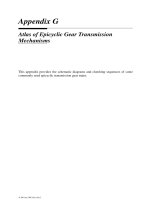
5.7 SQUEEZE-FILM FLOW
An example of the application of cylindrical coordinates to the squeeze-film
between two parallel, circular, concentric disks is shown in Fig. 5-5. The fluid
film between the two discs is very thin. The disks approach each other at a certain
speed. This results in a squeezing of the viscous thin film and in a radial pressure
distribution in the clearance and a load capacity that resists the motion of the
moving disk.
For a thin film, further simplification of the Navier–Stokes equations is
similar to that in the derivation of Eq. (5-10). The pressure is assumed to be
constant across the film thickness (in the z direction), and the dimension of z is
much smaller than that of r or rf. For a problem of radial symmetry, the Navier–
Stokes equations reduce to the following:
dp
dr
¼ m
@
2
v
r
@z
2
ð5-30Þ
Here, v
r
is the fluid velocity in the radial direction.
Example Problem 5-3
A fluid is squeezed between two parallel, circular, concentric disks, as shown in

Fig. 5-5. The fluid film between the two discs is very thin. The upper disk has
FIG. 5-5 Squeeze-film flow between two concentric, parallel disks.
Copyright 2003 by Marcel Dekker, Inc. All Rights Reserved.
velocity V, toward the lower disk, and this squeezes the fluid so that it escapes in
the radial direction. Derive the equations for the radial pressure distribution in the
thin film and the resultant load capacity.
Solution
The first step is to solve for the radial velocity distribution, v
r
, in the fluid film. In
a similar way to the hydrodynamic lubrication problem in the previous chapter,
we can write the differential equation in the form
@
2
v
r
@z
2
¼
dp
dr
1
m
¼ 2m
Here, m is a function of r only; m ¼ mðrÞ is a substitution that represents the
pressure gradient. By integration the preceding equation twice, the following
parabolic distribution of the radial velocity is obtained:
v
r
¼ mz

2
þ nz þ k
Here, m, n, and k are functions of r only. These functions are solved by the
boundary conditions of the radial velocity and the conservation of mass as well as
fluid volume for incompressible flow.
The two boundary conditions of the radial velocity are
at z ¼ 0: v
r
¼ 0
at z ¼ h: v
r
¼ 0
In order to solve for the three unknowns m, n and k, a third equation is required;
this is obtained from the fluid continuity, which is equivalent to the conservation
of mass.
Let us consider a control volume of a disk of radius r around the center of
the disk. The downward motion of the upper disk, at velocity V, reduces the
volume of the fluid per unit of time. The fluid is incompressible, and the
reduction of volume is equal to the radial flow rate Q out of the control
volume. The flow rate Q is the product of the area of the control volume pr
2
and the downward velocity V :
Q ¼ pr
2
V
The same flow rate Q must apply in the radial direction through the boundary of
the control volume. The flow rate Q is obtained by integration of the radial
velocity distribution of the film radial velocity, v
r
, along the z direction, multi-

plied by the circumference of the control volume ð2prÞ. The flow rate Q becomes
Q ¼ 2pr
ð
h
0
v
r
dz
Copyright 2003 by Marcel Dekker, Inc. All Rights Reserved.
Since the fluid is incompressible, the flow rate of the fluid escaping from the
control volume is equal to the flow rate of the volume displaced by the moving
disk:
V pr
2
¼ 2pr
ð
h
0
v
r
dz
Use of the boundary conditions and the preceding continuity equation allows the
solution of m, n, and k. The solution for the radial velocity distribution is
v
r
¼
3rV
h
z
2

h
2
À
z
h

and the pressure gradient is
)
dp
dr
¼À6mV
r
h
3
The negative sign means that the pressure is always decreasing in the r direction.
The pressure gradient is a linear function of the radial distance r, and this function
can be integrated to solve for the pressure wave:
p ¼
ð
dp ¼À
6mV
h
3
ð
rdr¼À
3mV
h
3
r
2

þ C
Here, C is a constant of integration that is solved by the boundary condition that
states that at the outside edge of the disks, the fluid pressure is equal to
atmospheric pressure, which can be considered to be zero:
at r ¼ R: p ¼ 0
Substituting in the preceding equation yields:
0 ¼À
3mV
h
3
R
2
þ C ) C ¼
3mV
h
3
R
2
The equation for the radial pressure distribution is therefore
) p ¼À
3mV
h
3
r
2
þ
3mV
h
3
R

2

¼
3mV
h
3
ðR
2
À r
2
Þ
The pressure has its maximum value at the center of the disk radius:
P
max
¼
3mV
h
3
½R
2
Àð0Þ
2
¼
3mV
h
3
R
2
The parabolic pressure distribution is shown in Fig. 5-6.
Copyright 2003 by Marcel Dekker, Inc. All Rights Reserved.

Solution
a. The viscosity of the lubricant is obtained from the viscosity–tempera-
ture chart:
m
SAE30@50

C
¼ 5:5 Â 10
À2
N-s=m
2
The film thickness is derived from the load capacity equation:
W ¼
3pmVR
4
2h
3
The instantaneous film thickness, when the disk speed is 10 m=s, is
h ¼
3p  5:5 Â10
À2
 10 Â15 Â10
À3
2 Â7000

1
3
h ¼ 0:266 mm
b. The maximum pressure at the center is
p

max
¼
3mV
h
3
R
2
¼
3ð5:5 Â 10
À2
N-s=m
2
Þð10 msÞð15 Â 10
À3
mÞ
2
ð0:266 Â10
À3
mÞ
3
¼ 1:97 Â 10
7
Pa ¼ 19:7 MPa
Problems
5-1 Two long cylinders of radii R
1
and R
2
, respectively, have parallel
centrelines, as shown in Fig. 5-7. The cylinders are submerged in

fluid and are rotating in opposite directions at angular speeds of o
1
and o
2
, respectively. The minimum clearance between the cylinders is
h
n
. If the fluid viscosity is m, derive the Reynolds equation, and write
the expression for the pressure gradient around the minimum clear-
ance.
The equation of the clearance is
hðxÞ¼h
n
þ
x
2
2R
eq
For calculation of the variable clearance between two cylinders
having a convex contact, the equation for the equivalent radius R
eq
is
1
R
eq
¼
1
R
1
þ

1
R
2
5-2 Two long cylinders of radii R
1
and R
2
, respectively, in concave contact
Copyright 2003 by Marcel Dekker, Inc. All Rights Reserved.
5-3 The journal diameter of a hydrodynamic bearing is d ¼ 100 mm, and
the radial clearance ratio is C=R ¼ 0:001. The journal speed is
N ¼ 20;000 RPM. The lubricant is mineral oil, SAE 30, at 70

C.
The lubricant density at the operating temperature is r ¼ 860 kg=m
3
.
a. Find the Reynolds number.
b. Find the journal speed, N , where instability in the form of
Taylor vortices initiates.
5-4 Two parallel circular disks of 100-mm diameter have a clearance of
1 mm between them. Under load, the downward velocity of the upper
disk is 2 m=s. At the same time, the lower disk is stationary. The
clearance is full of SAE 10 oil at a temperature of 60

C.
a. Find the load on the upper disk that results in the instanta-
neous velocity of 2 m=s.
b. What is the maximum pressure developed due to that load?
5-5 Two parallel circular disks (see Fig. 5-5) of 200-mm diameter have a

clearance of h ¼ 2 mm between them. The load on the upper disk is
200 N. The lower disk is stationary, and the upper disk has a
downward velocity V. The clearance is full of oil, SAE 10, at a
temperature of 60

C.
a. Find the downward velocity of the upper disk at that
instant.
b. What is the maximum pressure developed due to that load?
Copyright 2003 by Marcel Dekker, Inc. All Rights Reserved.
6
Long Hydrodynamic Journal
Bearings
6.1 INTRODUCTION
A hydrodynamic journal bearing is shown in Fig. 6-1. The journal is rotating
inside the bore of a sleeve with a thin clearance. Fluid lubricant is continuously
supplied into the clearance. If the journal speed is sufficiently high, pressure
builds up in the fluid film that completely separates the rubbing surfaces.
Hydrodynamic journal bearings are widely used in machinery, particularly
in motor vehicle engines and high-speed turbines. The sleeve is mounted in a
housing that can be a part of the frame of a machine. For successful operation, the
bearing requires high-precision machining. For most applications, the mating
surfaces of the journal and the internal bore of the bearing are carefully made with
precise dimensions and a good surface finish.
The radial clearance, C, between the bearing bore of radius R
1
and of the
journal radius, R,isC ¼ R
1
À R (see Fig. 6-1). In most practical cases, the

clearance, C, is very small relative to the journal radius, R. The following order of
magnitude is applicable for most design purposes:
C
R
% 10
À3
ð6-1Þ
A long hydrodynamic bearing is where the bearing length, L, is long in
comparison to the journal radius ðL ) RÞ. Under load, the center of the journal,
Copyright 2003 by Marcel Dekker, Inc. All Rights Reserved.
particularly in a high-speed journal bearing. Therefore, for proper design, the
bearing must operate at eccentricity ratios well below 1, to allow adequate
minimum film thickness to separate the sliding surfaces. Most journal bearings
operate under steady conditions in the range from e ¼ 0:6toe ¼ 0:8. However,
the most important design consideration is to make sure the minimum film
thickness, h
n
, will be much higher than the size of surface asperities or the level
of journal vibrations during operation.
6.2 REYNOLDS EQUATION FOR A JOURNAL
BEARING
In Chapter 4, the hydrodynamic equations of a long journal bearing were derived
from first principles. In this chapter, the hydrodynamic equations are derived from
the Reynolds equation. The advantage of the present approach is that it can apply
to a wider range of problems, such as bearings under dynamic conditions.
Let us recall that the general Reynolds equation for a Newtonian incom-
pressible thin fluid film is
@
@x
h

3
m
@p
@x

þ
@
@z
h
3
m
@p
@z

¼ 6ðU
1
À U
2
Þ
@h
@x
þ 12ðV
2
À V
1
Þð6-5Þ
Here, U
1
and U
2

are velocity components, in the x direction, of the lower and
upper sliding surfaces, respectively (fluid film boundaries), while the velocities
components V
1
and V
2
are of the lower and upper boundaries, respectively, in the
y direction (see Fig. 5-2). The difference in normal velocity ðV
1
À V
2
Þ is of
relative motion (squeeze-film action) of the surfaces toward each other.
For most journal bearings, only the journal is rotating and the sleeve is
stationary, U
1
¼ 0; V
1
¼ 0 (as shown in Fig. 6-1). The second fluid film boundary
is at the journal surface that has a velocity U ¼ oR. However, the velocity U is
not parallel to the x direction (the x direction is along the bearing surface).
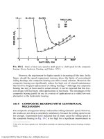
FIG. 6-2 Velocity components of the fluid film boundaries.
Copyright 2003 by Marcel Dekker, Inc. All Rights Reserved.
Therefore, it has two components (as shown in Fig. 6-2), U
2
and V
2
, in the x and y
directions, respectively:
U

2
¼ U cos a
V
2
¼ÀU sin a
ð6-6Þ
Here, the slope a is between the bearing and journal surfaces. In a journal
bearing, the slope a is very small; therefore, the following approximations can be
applied:
U
2
¼ U cos a % U
V
2
¼ÀU sin a %ÀU tan a
ð6-7Þ
The slope a can be expressed in terms of the function of the clearance, h:
tan a ¼À
@h
@x
ð6-8Þ
The normal component V
2
becomes
V
2
% U
@h
@x
ð6-9Þ

After substituting Eqs. (6.7) and (6.9) into the right-hand side of the Reynolds
equation, it becomes
6ðU
1
À U
2
Þ
@h
@x
þ 12ðV
2
À V
1
Þ¼6ð0 ÀUÞ
@h
@x
þ 12U
@h
@x
¼ 6U
@h
@x
ð6-10Þ
The Reynolds equation for a Newtonian incompressible fluid reduces to the
following final equation:
@
@x
h
3
m

@p
@x

þ
@
@z
h
3
m
@p
@z

¼ 6U
@h
@x
ð6-11Þ
For an infinitely long bearing, @p=@z ffi 0; therefore, the second term on the left-
hand side of Eq. (6-11) can be omitted, and the Reynolds equation reduces to the
following simplified one-dimensional equation:
@
@x
h
3
m
@p
@x

¼ 6U
@h
@x

ð6-12Þ
6.3 JOURNAL BEARING WITH ROTATING
SLEEVE
There are many practical applications where the sleeve is rotating as well as the
journal. In that case, the right-hand side of the Reynolds equation is not the same
as for a common stationary bearing. Let us consider an example, as shown in Fig.
Copyright 2003 by Marcel Dekker, Inc. All Rights Reserved.
6-3, where the sleeve and journal are rolling together like internal friction pulleys.
The rolling is similar to that in a cylindrical rolling bearing. The internal sleeve
and journal surface are rolling together without slip, and both have the same
tangential velocity o
j
R ¼ o
b
R
1
¼ U.
The tangential velocities of the film boundaries, in the x direction, of the
two surfaces are
U
1
¼ U
U
2
¼ U cos a % U
ð6-13Þ
The normal velocity components, in the y direction, of the film boundaries (the
journal and sleeve surfaces) are
V
1

¼ 0
V
2
% U
@h
@x
ð6-14Þ
The right-hand side of the Reynolds equation becomes
6ðU
1
À U
2
Þ
@h
@x
þ 12ðV
2
À V
1
Þ¼6ðU À U Þ
@h
@x
þ 12ðU
@h
@x
À 0Þ¼12U
@h
@x
ð6-15Þ
For the rolling action, the Reynolds equation for a journal bearing with a rolling

sleeve is given by
@
@x
h
3
m
@p
@x

þ
@
@z
h
3
m
@p
@z

¼ 12U
@h
@x
ð6-16Þ
The right-hand side of Eq. (6-16) indicates that the rolling action will result in a
doubling of the pressure wave of a common journal bearing of identical geometry
as well as a doubling its load capacity. The physical explanation is that the fluid is
squeezed faster by the rolling action.
6.4 COMBINED ROLLING AND SLIDING
In many important applications, such as gears, there is a combination of rolling
and sliding of two cylindrical surfaces. Also, there are several unique applications
where a hydrodynamic journal bearing operates in a combined rolling-and-sliding

mode. A combined bearing is shown in Fig. 6-3, where the journal surface
velocity is Ro
j
while the sleeve inner surface velocity is R
1
o
b
.
The coefficient x is the ratio of the rolling and sliding velocity. In terms of
the velocities of the two surfaces, the ratio is,
x ¼
R
1
o
b
Ro
j
ð6-17Þ
Copyright 2003 by Marcel Dekker, Inc. All Rights Reserved.