Bearing Design in Machinery Episode 1 Part 6 ppt

Here, L is the width of the parallel plates, in the direction normal to the flow (in
the z direction). Substituting the flow in Eq. (4-29) into Eq. (4-30) and integrating
yields the expression for the pressure gradient as a function of flow rate, Q:
dp
dx
¼À
12m
bh
3
0
Q ð4-31Þ
This equation is useful for the hydrostatic bearing calculations in Chapter 10. The
negative sign means that a negative pressure slope in the x direction is required
for a flow in the same direction.
4.10 FLUID FILM BETWEEN A CYLINDER AND A
FLAT PL ATE
There are important applications of a full fluid film at the rolling contact of a
cylinder and a flat plate and at the contact of two parallel cylinders. Examples are
cylindrical rolling bearings, cams, and gears. A very thin fluid film that separates
the surfaces is shown in Fig. 4-7. In this example, the cylinder is stationary and
the flat plate has a velocity U in the x direction. In Chapter 6, this problem is
extended to include rolling motion of the cylinder over the plate.
The problem of a cylinder and a flat plate is a special case of the general
problem of contact between two parallel cylinders. By using the concept of
equivalent radius (see Chapter 12), the equations for a cylinder and a flat plate can
be extended to that for two parallel cylinders.
Fluid films at the contacts of rolling-element bearings and gear teeth are
referred to as elastohydrodynamic (EHD) films. The complete analysis of a fluid
film in actual rolling-element bearings and gear teeth is quite complex. Under
load, the high contact pressure results in a significant elastic deformation of the
contact surfaces as well as a rise of viscosity with pressure (see Chapter 12).

FIG. 4.7 Fluid film between a cylinder and a flat-plate.
Copyright 2003 by Marcel Dekker, Inc. All Rights Reserved.
However, the following problem is for a light load where the solid surfaces are
assumed to be rigid and the viscosity is constant.
The following problem considers a plate and a cylinder with a minimum
clearance, h
min
. In it we consider the case of a light load, where the elastic
deformation is very small and can be disregarded (cylinder and plate are assumed
to be rigid). In addition, the values of maximum and minimum pressures are
sufficiently low, and there is no fluid cavitation. The viscosity is assumed to be
constant. The cylinder is stationary, and the flat plate has a velocity U in the x
direction as shown in Fig. 4-7.
The cylinder is long in comparison to the film length, and the long-bearing
analysis can be applied.
4.10.1 Film Thickness
The film thickness in the clearance between a flat plate and a cylinder is given by
hðyÞ¼h
min
þ Rð1 Àcos yÞð4-32Þ
where y is a cylinder angle measured from the minimum film thickness at x ¼ 0.
Since the minimum clearance, h
min
, is very small (relative to the cylinder
radius), the pressure is generated only at a very small region close to the
minimum film thickness, where x ( R,orx=R ( 1.
For a small ratio of x=R, the equation of the clearance, h, can be
approximated by a parabolic equation. The following expression is obtained by
expanding Eq. (4-32) for h into a Taylor series and truncating terms that include
powers higher than ðx=RÞ

2
. In this way, the expression for the film thickness h can
be approximated by
hðxÞ¼h
min
þ
x
2
2R
ð4-33aÞ
4.10.2 Pressure Wave
The pressure wave can be derived from the expression for the pressure gradient,
dp=dx, in Eq. (4-13). The equation is
dp
dx
¼ 6mU
h
0
À h
h
3
The unknown h
0
can be replaced by the unknown x
0
according to the equation
h
0
ðxÞ¼h
min

þ
x
2
0
2R
ð4-33bÞ
Copyright 2003 by Marcel Dekker, Inc. All Rights Reserved.
After substituting the value of h according to Eqs. (4-33), the solution for the
pressure wave can be obtained by the following integration:
pðxÞ¼24mUR
2
ð
x
À1
x
2
0
À x
2
ð2Rh
min
þ x
2
Þ
3
dx ð4-34Þ
The unknown x
0
is solved by the following boundary conditions of the pressure
wave:

at x ¼À1: p ¼ 0
at x ¼1: p ¼ 0
ð4-35Þ
For numerical integration, the infinity can be replaced by a relatively large finite
value, where pressure is very small and can be disregarded.
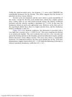
Remark: The result is an antisymmetrical pressure wave (on the two sides
of the minimum film thickness), and there will be no resultant load capacity. In
actual cases, the pressures are high, and there is a cavitation at the diverging side.
A solution that considers the cavitation with realistic boundary conditions is
presented in Chapter 6.
4.11 SOLUTION IN DIMENSIONLESS TERMS
If we perform a numerical integration of Eq. (4-34) for solving the pressure wave,
the solution would be limited to a specific bearing geometry of cylinder radius R
and minimum clearance h
min
. The numerical integration must be repeated for a
different bearing geometry.
For a universal solution, there is obvious merit to performing a solution in
dimensionless terms. For conversion to dimensionless terms, we normalize the x
coordinate by dividing it by
ffiffiffiffiffiffiffiffiffiffiffiffiffiffi
2Rh
min
p
and define a dimensionless coordinate as
"
xx ¼
x
ffiffiffiffiffiffiffiffiffiffiffiffiffiffi
2Rh

min
p
ð4-36Þ
In addition, a dimensionless clearance ratio is defined:
"
hh ¼
h
h
min
ð4-37Þ
The equation for the variable clearance ratio as a function of the dimensionless
coordinate becomes
"
hh ¼ 1 þ
"
xx
2
ð4-38Þ
Copyright 2003 by Marcel Dekker, Inc. All Rights Reserved.
Let us recall that the unknown h
0
is the fluid film thickness at the point of peak
pressure. It is often convenient to substitute it by the location of the peak pressure,
x
0
, and the dimensionless relation then is
"
hh
0
¼ 1 þ

"
xx
2
0
ð4-39Þ
In addition, if the dimensionless pressure is defined as
"
pp ¼
h
2
min
ffiffiffiffiffiffiffiffiffiffiffiffiffiffi
2Rh
min
p
1
6mU
p ð4-40Þ
then the following integration gives the dimensionless pressure wave:
"
pp ¼
ð
d
"
pp ¼
ð
"
xx
À1
"

xx
2
À
"
xx
2
0
ð1 þ
"
xx
2
Þ
3
d
"
xx ð4-41Þ
For a numerical integration of the pressure wave according to Eq. (4-41), the
boundary
"
xx ¼À1is replaced by a relatively large finite dimensionless value,
where pressure is small and can be disregarded, such as
"
xx ¼À4. An example of
numerical integration is given in Example Problem 4.
In a similar way, for a numerical solution of the unknown x
0
and the load
capacity, it is possible to replace infinity with a finite number, for example, the
following mathematical boundary conditions of the pressure wave of a full fluid
film between a cylinder and a plane:

at
"
xx ¼À1:
"
pp ¼ 0
at
"
xx ¼1:
"
pp ¼ 0
ð4-42aÞ
These conditions are replaced by practical numerical boundary conditions:
at
"
xx ¼À4:
"
pp ¼ 0
at
"
xx ¼þ4:
"
pp ¼ 0
ð4-42bÞ
These practical numerical boundary conditions do not introduce a significant
error because a significant hydrodynamic pressure is developed only near the
minimum fluid film thickness, at
"
xx ¼ 0.
Example Problem 4-4
Ice Sled

An ice sled is shown in Fig. 4-8. On the left-hand side, there is a converging
clearance that is formed by the geometry of a quarter of a cylinder. A flat plate
continues the curved cylindrical shape. The flat part of the sled is parallel to the
flat ice. It is running parallel over the flat ice on a thin layer of water film of a
constant thickness h
0
.
Copyright 2003 by Marcel Dekker, Inc. All Rights Reserved.
Derive and plot the pressure wave at the entrance region of the fluid film
and under the flat ice sled as it runs over the ice at velocity U. Derive the equation
of the sled load capacity.
Solution
The long-bearing approximation is assumed for the sled similar to the converging
slope in Fig. 4-4. The fluid film equation for an infinitely long bearing is
dp
dx
¼ 6mU
h À h
0
h
3
In the parallel region, h ¼ h
0
, and it follows from the foregoing equation that
dp
dx
¼ 0 ðalong the parallel region of constant clearanceÞ
In this case, h
0
¼ h

min
, and the equation for the variable clearance at the
converging region is
hðxÞ¼h
0
þ
x
2
2R
This means that for a wide sled, the pressure is constant within the parallel region.
This is correct only if L ) B, where L is the bearing width (in the z direction) and
B is along the sled in the x direction.
Fluid flow in the converging region generates the pressure, which is
ultimately responsible for supporting the load of the sled. Through the adhesive
force of viscous shear, the fluid is dragged into the converging clearance, creating
the pressure in the parallel region.
Substituting hðxÞ into the pressure gradient equation yields
dp
dx
¼ 6mU
h
0
þ
x
2
2R

À h
0
h

0
þ
x
2
2R

3
or
dp
dx
¼ 24mUR
2
x
2
ð2Rh
0
þ x
2
Þ
3
Applying the limits of integration and the boundary condition, we get the
following for the pressure distribution:
pðxÞ¼24mUR
2
ð
x
À1
x
2
ð2Rh

0
þ x
2
Þ
3
dx
Copyright 2003 by Marcel Dekker, Inc. All Rights Reserved.
This equation can be integrated analytically or numerically. For numerical
integration, since a significant pressure is generated only at a low x value, the
infinity boundary of integration is replaced by a finite magnitude.
Conversion to a Dimensionless Equation. As discussed earlier, there is an
advantage in solving the pressure distribution in dimensionless terms. A regular
pressure distribution curve is limited to the specific bearing data of given radius R
and clearance h
0
. The advantage of a dimensionless curve is that it is universal
and applies to any bearing data. For conversion of the pressure gradient to
dimensionless terms, we normalize x by dividing by
ffiffiffiffiffiffiffiffiffiffi
2Rh
0
p
and define dimen-
sionless terms as follows:
"
xx ¼
x
ffiffiffiffiffiffiffiffiffiffi
2Rh
0

p
;
"
hh ¼
h
h
0
;
"
hh ¼ 1 þ
"
xx
2
Converting to dimensionless terms, the pressure gradient equation gets the form
dp
dx
¼
6mU
h
2
0
"
hh À 1
ð1 þ
"
xx
2
Þ
3
Here, h

0
¼ h
min
is the minimum film thickness at x ¼ 0. Substituting for the
dimensionless clearance and rearranging yields
h
2
0
ffiffiffiffiffiffiffiffiffiffi
2Rh
0
p
6mU
dp ¼
"
xx
2
ð1 þ
"
xx
2
Þ
3
dx
The left-hand side of this equation is defined as the dimensionless pressure.
Dimensionless pressure is equal to the following integral:
"
pp ¼
h
2

0
ffiffiffiffiffiffiffiffiffiffi
2Rh
0
p
1
6mU
ð
p
0
dp ¼
ð
x
À1
"
xx
2
ð1 þ
"
xx
2
Þ
3
d
"
xx
Numerical Integration. The dimensionless pressure is solved by an
analytical or numerical integration of the preceding function within the specified
boundaries (see Appendix B). The pressure p
0

under the flat plate is obtained by
integration to the limit x ¼ 0:
"
pp ¼
h
2
0
ffiffiffiffiffiffiffiffiffiffi
2Rh
0
p
1
6mU
p
0
¼
X
x
À3
x
2
i
ð1 þx
2
i
Þ
3
Dx
i
The pressure is significant only near x ¼ 0. Therefore, for the numerical

integration, a finite number replaces infinity. The resulting pressure distribution
is shown in Fig. 4-9.
Comparison with Analytical Integration. The maximum pressure at x ¼ 0
as well as along the constant clearance, x > 0, can also be solved by analytical
Copyright 2003 by Marcel Dekker, Inc. All Rights Reserved.
If the load, cylinder radius, water viscosity, and sled velocity are known, it is
possible to solve for the film thickness, h
0
.
Example Problem 4-5
Derive the equation for the pressure gradient of a journal bearing if the journal
and bearing are both rotating around their stationary centers. The surface velocity
of the bearing bore is U
j
; ¼ o
j
R, and the surface velocity of the journal is
U
b
¼ o
b
R
1
.
Solution
Starting from Eq. (4-4):
dp
dx
¼ m
@

2
u
@y
2
and integrating twice (in a similar way to a stationary bearing) yields
u ¼ my
2
þ ny þk
However, the boundary conditions and continuity conditions are as follows:
at y ¼ 0: u ¼ o
b
R
1
at y ¼ hð xÞ: u ¼ o
j
R
In this case, the constant-volume flow rate, q, per unit of bearing length at
the point of peak pressure is
q ¼
ð
h
0
udy¼
ðo
b
R
1
þ o
j
RÞh

0
2
Solving for m, n and k and substituting in a similar way to the previous problem
while also assuming R
1
% R, the following equation for the pressure gradient is
obtained:
dp
dx
¼ 6Rðo
b
þ o
j
Þm
h À h
0
h
3
Problems
4-1 A long plane-slider, L ¼ 200 mm and B ¼ 100 mm, is sliding at
velocity of 0.3 m=s. The minimum film thickness is h
1
¼ 0:005 mm
and the maximum film thickness is h
2
¼ 0:010 mm. The fluid is SAE
30, and the operating temperature of the lubricant is assumed a
constant 30

C.

a. Assume the equation for an infinitely long bearing, and use
numerical integration to solve for the pressure wave (use
Copyright 2003 by Marcel Dekker, Inc. All Rights Reserved.
trial and error to solve for x
0
). Plot a curve of the pressure
distribution p ¼ pðxÞ.
b. Use numerical integration to find the load capacity.
Compare this to the load capacity obtained from Eq. (4-
19).
c. Find the friction force and the friction coefficient.
4-2 A slider is machined to have a parabolic surface. The slider has a
horizontal velocity of 0.3 m=s. The minimum film h
min
¼ 0:020 mm,
and the clearance varies with x according to the following equation:
h ¼ 0:020 þ 0:01x
2
The slider velocity is U ¼ 0:5m=s. The length L ¼ 300 mm
and the width in the sliding direction B ¼ 100 mm. The lubricant is
SAE 40 and the temperature is assumed constant, T ¼ 40

C. Assume
the equation for an infinitely long bearing.
a. Use numerical integration and plot the dimensionless
pressure distribution, p ¼ pðxÞ.
b. Use numerical integration to find the load capacity.
c. Find the friction force and the friction coefficient.
4-3 A blade of a sled has the geometry shown in the Figure 4-8. The sled
is running over ice on a thin layer of water film. The total load (weight

of the sled and person) is 1500 N. The sled velocity is 20 km=h, the
radius of the inlet curvature is 30 cm, and the sled length B ¼ 30 cm,
and width is L ¼ 100 cm. The viscosity of water is m ¼ 1:792Â
10
À3
N-s=m
2
.
Find the film thickness ðh
0
¼ h
min
Þ of the thin water layer shown in
Fig. 4-8.
Direction: The clearance between the plate and disk is
h ¼ h
min
þ x
2
=2R, and assume that p ¼ 0atx ¼ R.
Copyright 2003 by Marcel Dekker, Inc. All Rights Reserved.
5
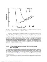
Basic Hydrodynamic Equations
5.1 NAVIER^STOKES EQUATIONS
The pressure distribution and load capacity of a hydrodynamic bearing are
analyzed and solved by using classical fluid dynamics equations. In a thin fluid
film, the viscosity is the most important fluid property determining the magnitude
of the pressure wave, while the effect of the fluid inertia (ma) is relatively small
and negligible. Reynolds (1894) introduced classical hydrodynamic lubrication
theory. Although a lot of subsequent research has been devoted to this discipline,

Reynolds’ equation still forms the basis of most analytical research in hydro-
dynamic lubrication. The Reynolds equation can be derived from the Navier–
Stokes equations, which are the fundamental equations of fluid motion.
The derivation of the Navier–Stokes equations is based on several assump-
tions, which are included in the list of assumptions (Sec. 4.2) that forms the basis
of the theory of hydrodynamic lubrication. An important assumption for the
derivation of the Navier–Stokes equations is that there is a linear relationship
between the respective components of stress and strain rate in the fluid.
In the general case of three-dimensional flow, there are nine stress
components referred to as components of the stress tensor. The directions of
the stress components are shown in Fig 5-1.
Copyright 2003 by Marcel Dekker, Inc. All Rights Reserved.
is an adequate approximation. However, under extreme conditions, e.g., very high
pressure of point or line contacts, this assumption is no longer valid. An
assumption that is made for convenience is that the viscosity, m, of the lubricant
is constant. Also, lubrication oils are practically incompressible, and this property
simplifies the Navier–Stokes equations because the density, r, can be assumed to
be constant. However, this assumption cannot be applied to air bearings.
Comment. As mentioned earlier, in thin films the velocity component n is
small in comparison to u and w, and two shear components can be approximated
as follows:
t
xy
¼ t
yx
¼ m
@v
@x
þ
@u

@y

% m
@u
@y
t
yz
¼ t
zy
¼ m
@w
@y
þ
@v
@z

% m
@w
@y
ð5-3Þ
The Navier–Stokes equations are based on the balance of forces acting on a
small, infinitesimal fluid element having the shape of a rectangular parallelogram
with dimensions dx, dy, and dz, as shown in Fig. 5-1. The force balance is similar
to that in Fig. 4-1; however, the general balance of forces is of three dimensions,
in the x; y and z directions. The surface forces are the product of stresses, or
pressures, and the corresponding areas.
When the fluid is at rest there is a uniform hydrostatic pressure. However,
when there is fluid motion, there are deviatoric normal stresses s
0
x

, s
0
y
, s
0
z
that are
above the hydrostatic (average) pressure, p. Each of the three normal stresses is
the sum of the average pressure, and the deviatoric normal stress (above the
average pressure), as follows:
s
x
¼Àp þs
0
x
; s
y
¼Àp þs
0
y
; s
z
¼Àp þs
0
z
ð5-4aÞ
According to Newton’s second law, the sum of all forces acting on a fluid
element, including surface forces in the form of stresses and body forces such as
the gravitational force, is equal to the product of mass and acceleration (ma)of
the fluid element. After dividing by the volume of the fluid element, the equations

of the force balance become
r
du
dt
¼ X À
@p
@x
þ
@s
0
x
@x
þ
@t
xy
@y
þ
@
xz
@z
r
dv
dt
¼ Y À
@p
@y
þ
@t
yx
@y

þ
@s
0
y
@y
þ
@t
yz
@z
ð5-4bÞ
r
dw
dt
¼ Z À
@p
@z
þ
@t
zx
@x
þ
@t
zy
@y
þ
@s
0
z
@z
Copyright 2003 by Marcel Dekker, Inc. All Rights Reserved.

Here, p is the pressure, u, v, and w are the velocity components in the x, y,
and z directions, respectively. The three forces X ; Y ; Z are the components of a
body force, per unit volume, such as the gravity force that is acting on the fluid.
According to the assumptions, the fluid density, r, and the viscosity, m, are
considered constant. The derivation of the Navier–Stokes equations is included in
most fluid dynamics textbooks (e.g., White, 1985).
For an incompressible flow, the continuity equation, which is derived from
the conservation of mass, is
@u
@x
þ
@v
@y
þ
@w
@z
¼ 0 ð5-5Þ
After substituting the stress components of Eq. (5-2) into Eq. (5-4b), using
the continuity equation (5-5) and writing in full the convective time derivative of
the acceleration components, the following Navier–Stokes equations in Cartesian
coordinates for a Newtonian incompressible and constant-viscosity fluid are
obtained
r
@u
@t
þ u
@u
@x
þ v
@u

@y
þ w
@u
@z

¼ X À
@p
@x
þ m
@
2
u
@x
2
þ
@
2
u
@y
2
þ
@
2
u
@z
2

ð5-6aÞ
r
@v

@t
þ u
@v
@x
þ v
@v
@y
þ w
@v
@z

¼ Y ¼À
@p
@y
þ m
@
2
v
@x
2
þ
@
2
v
@y
2
þ
@
2
v

@z
2

ð5-6bÞ
r
@w
@t
þ u
@w
@x
þ v
@w
@y
þ w
@w
@z

¼ Z À
@p
@z
þ m
@
2
w
@x
2
þ
@
2
w

@y
2
þ
@
2
w
@z
2

ð5-6cÞ
The Navier–Stokes equations can be solved for the velocity distribution. The
velocity is described by its three components, u, v, and w, which are functions of
the location (x, y, z) and time. In general, fluid flow problems have four
unknowns: u, v, and w and the pressure distribution, p. Four equations are
required to solve for the four unknown functions. The equations are the three
Navier–Stokes equations, the fourth equation is the continuity equation (5-5).
5.2 REYNOLDS HYDRODYNAMIC LUBRICATION
EQUATION
Hydrodynamic lubrication involves a thin-film flow, and in most cases the fluid
inertia and body forces are very small and negligible in comparison to the viscous
forces. Therefore, in a thin-film flow, the inertial terms [all terms on the left side
of Eqs. (5.6)] can be disregarded as well as the body forces X , Y , Z. It is well
known in fluid dynamics that the ratio of the magnitude of the inertial terms
relative to the viscosity terms in Eqs. (5-6) is of the order of magnitude of the
Copyright 2003 by Marcel Dekker, Inc. All Rights Reserved.
Reynolds number, Re. For a lubrication flow (thin-film flow), Re ( 1, the
Navier–Stokes equations reduce to the following simple form:
@p
@x
¼ m

@
2
u
@x
2
þ
@
2
u
@y
2
þ
@
2
u
@z
2

ð5-7aÞ
@p
@y
¼ m
@
2
v
@x
2
þ
@
2

v
@y
2
þ
@
2
v
@z
2

ð5-7bÞ
@p
@z
¼ m
@
2
w
@x
2
þ
@
2
w
@y
2
þ
@
2
w
@z

2

ð5-7cÞ
These equations indicate that viscosity is the dominant effect in determining the
pressure distribution in a fluid film bearing.
The assumptions of classical hydrodynamic lubrication theory are summar-
ized in Chapter 4. The velocity components of the flow in a thin film are primarily
u and w in the x and z directions, respectively. These directions are along the fluid
film layer (see Fig. 1-2). At the same time, there is a relatively very slow velocity
component, v, in the y direction across the fluid film layer. Therefore, the pressure
gradient in the y direction in Eq. (5-7b) is very small and can be disregarded.
In addition, Eqs. (5-7a and c) can be further simplified because the order of
magnitude of the dimensions of the thin fluid film in the x and z directions is
much higher than that in the y direction across the film thickness. The orders of
magnitude are
x ¼ OðBÞ
y ¼ OðhÞ
z ¼ OðLÞ
ð5-8aÞ
Here, the symbol O represents order of magnitude. The dimension B is the
bearing length along the direction of motion (x direction), and h is an average
fluid film thickness. The width L is in the z direction of an inclined slider. In a
journal bearing, L is in the axial z direction and is referred to as the bearing
length.
In hydrodynamic bearings, the fluid film thickness is very small in com-
parison to the bearing dimensions, h ( B and h ( L. By use of Eqs. (5-8b), a
comparison can be made between the orders of magnitude of the second
Copyright 2003 by Marcel Dekker, Inc. All Rights Reserved.
derivatives of the various terms on the right-hand side of Eq. (5-7a), which are as
follows:

@
2
u
@y
2
¼ O
U
h
2

@
2
u
@x
2
¼ O
U
B
2

@
2
u
@z
2
¼ O
U
L
2


ð5-8bÞ
In conventional finite-length bearings, the ratios of dimensions are of the
following orders:
L
B
¼ Oð1Þ
h
B
¼ Lð10
À3
Þ
ð5-9Þ
Equations (5-8) and (5-9) indicate that the order of the term @
2
u=@y
2
is larger by
10
6
, in comparison to the order of the other two terms, @
2
u=@x
2
and @
2
u=@z
2
.
Therefore, the last two terms can be neglected in comparison to the first one in
Eq. (5-7a). In the same way, only the term @

2
w=@y
2
is retained in Eq. (5-7c).
According to the assumptions, the pressure gradient across the film thickness,
@p=@y, is negligible, and the Navier–Stokes equations reduce to the following two
simplified equations:
@p
@x
¼ m
@
2
u
@y
2
and
@p
@z
¼ m
@
2
w
@y
2
ð5-10Þ
The first equation is identical to Eq. (4-4), which was derived from first principles
in Chapter 4 for an infinitely long bearing. In a long bearing, there is a significant
pressure gradient only in the x direction; however, for a finite-length bearing,
there is a pressure gradient in the x and z directions, and the two Eqs. (5-10) are
required for solving the flow and pressure distributions.

The two Eqs. (5-10) together with the continuity Eq. (5-5) and the
boundary condition of the flow are used to derive the Reynolds equation. The
derivation of the Reynolds equation is included in several books devoted to the
analysis of hydrodynamic lubrication see Pinkus (1966), and Szeri (1980). The
Reynolds equation is widely used for solving the pressure distribution of
hydrodynamic bearings of finite length. The Reynolds equation for Newtonian
Copyright 2003 by Marcel Dekker, Inc. All Rights Reserved.
incompressible and constant-viscosity fluid in a thin clearance between two rigid
surfaces of relative motion is given by
@
@x
h
3
m
@p
@x

þ
@
@z
h
3
m
@p
@z

¼6ðU
1
À U
2

Þ
@h
@x
þ 6
@
@x
ðU
1
þ U
2
Þþ12ðV
2
À V
1
Þ
ð5-11Þ
The velocity components of the two surfaces that form the film boundaries
are shown in Fig. 5-2. The tangential velocity components, U
1
and U
2
, in the x
direction are of the lower and upper sliding surfaces, respectively (two fluid film
boundaries). The normal velocity components, in the y direction, V
1
and V
2
, are
of the lower and upper boundaries, respectively. In a journal bearing, these
components are functions of x (or angle y) around the journal bearing.

The right side of Eq. (5-11) must be negative in order to result in a positive
pressure wave and load capacity. Each of the three terms on the right-hand side of
Eq. (5-11) has a physical meaning concerning the generation of the pressure
wave. Each term is an action that represents a specific type of relative motion of
the surfaces. Each action results in a positive pressure in the fluid film. The
various actions are shown in Fig. 5-3. These three actions can be present in a
bearing simultaneously, one at a time or in any other combination. The following
are the various actions.
Viscous wedge action: This action generates positive pressure wave by
dragging the viscous fluid into a converging wedge.
Elastic stretching or compression of the boundary surface: This action
generates a positive pressure by compression of the boundary. The
compression of the surface reduces the clearance volume and the viscous
fluid is squeezed out, resulting in a pressure rise. This action is
FIG. 5-2 Directions of the velocity components of fluid-film boundaries in the
Reynolds equation.
Copyright 2003 by Marcel Dekker, Inc. All Rights Reserved.
bearing material. This action is usually not considered for rigid bearing
materials.
Squeeze-film action: The squeezing action generates a positive pressure by
reduction of the fluid film volume. The incompressible viscous fluid is
squeezed out through the thin clearance. The thin clearance has
resistance to the squeeze-film flow, resulting in a pressure buildup to
overcome the flow resistance (see Problem 5-3).
In most practical bearings, the surfaces are rigid and there is no stretching
or compression action. In that case, the Reynolds equation for an incompressible
fluid and constant viscosity reduces to
@
@x
h

3
m
@p
@x

þ
@
@z
h
3
m
@p
@z

¼ 6ðU
1
À U
2
Þ
@h
@x
þ 12ðV
2
À V
1
Þð5-12Þ
As indicated earlier, the two right-hand terms must be negative in order to
result in a positive pressure wave. On the right side of the Reynolds equation, the
first term of relative sliding motion ðU
1

À U
2
Þ describes a viscous wedge effect. It
requires inclined surfaces, @h=@x, to generate a fluid film wedge action that results
in a pressure wave. Positive pressure is generated if the film thickness reduces in
the x direction (negative @h=@x).
The second term on the right side of the Reynolds equation describes a
squeeze-film action. The difference in the normal velocity ðV
2
À V
1
Þ represents
the motion of surfaces toward each other, referred to as squeeze-film action.A
positive pressure builds up if ðV
2
À V
1
Þ is negative and the surfaces are
approaching each other. The Reynolds equation indicates that a squeeze-film
effect is a viscous effect that can generate a pressure wave in the fluid film, even
in the case of parallel boundaries.
It is important to mention that the Reynolds equation is objective, in the
sense that the pressure distribution must be independent of the selection of the
coordinate system. In Fig. 5-2 the coordinates are stationary and the two surfaces
are moving relative to the coordinate system. However, the same pressure
distribution must result if the coordinates are attached to one surface and are
moving and rotating with it. For convenience, in most problems we select a
stationary coordinate system where the x coordinate is along the bearing surface
and the y coordinate is normal to this surface. In that case, the lower surface has
only a tangential velocity, U

1
, and there is no normal component, V
1
¼ 0.
The value of each of the velocity components of the fluid boundary, U
1
, U
2
,
V
1
, V
2
, depends on the selection of the coordinate system. Surface velocities in a
stationary coordinate system would not be the same as those in a moving
coordinate system. However, velocity differences on the right-hand side of the
Reynolds equation, which represent relative motion, are independent of the
selection of the coordinate system. In journal bearings under dynamic conditions,
Copyright 2003 by Marcel Dekker, Inc. All Rights Reserved.
the journal center is not stationary. The velocity of the center must be considered
for the derivation of the right-hand side terms of the Reynolds equation.
5.3 WIDE PLANE-SLIDER
The equation of a plane-slider has been derived from first principles in Chapter 4.
Here, this equation will be derived from the Reynolds equation and compared to
that in Chapter 4.
A plane-slider and its coordinate system are shown in Fig. 1-2. The lower
plate is stationary, and the velocity components at the lower wall are U
1
¼ 0 and
V

1
¼ 0. At the same time, the velocity at the upper wall is equal to that of the
slider. The slider has only a horizontal velocity component, U
2
¼ U , where U is
the plane-slider velocity. Since the velocity of the slider is in only the x direction
and there is no normal component in the y direction, V
2
¼ 0. After substituting
the velocity components of the two surfaces into Eq. (5-11), the Reynolds
equation will reduce to the form
@
@x
h
3
m
@p
@x

þ
@
@z
h
3
m
@p
@z

¼ 6U
@h

@x
ð5-13Þ
For a wide bearing, L ) B,wehave@p=@z ffi 0, and the second term on the left
side of Eq. (5-13) can be omitted. The Reynolds equation reduces to the
following simplified form:
@
@x
h
3
m
@p
@x

¼ 6U
@h
@x
ð5-14Þ
For a plane-slider, if the x coordinate is in the direction of a converging clearance
(the clearance reduces with x), as shown in Fig. 4-4, integration of Eq. (5-14)
results in a pressure gradient expression equivalent to that of a hydrodynamic
journal bearing or a negative-slope slider in Chapter 4. The following equation is
the expression for the pressure gradient for a converging clearance, @h=@x < 0
(negative slope):
dp
dx
¼ 6U m
h À h
0
h
3

for initial
@h
@x
< 0 ðnegative slope in Fig: 4-4Þ
ð5-15Þ
The unknown constant h
0
(constant of integration) is determined from additional
information concerning the boundary conditions of the pressure wave. The
meaning of h
0
is discussed in Chapter 4—it is the film thickness at the point
of a peak pressure along the fluid film. In a converging clearance such as a journal
bearing near x ¼ 0, the clearance slope is negative, @h=@x < 0. The result is that
the pressure increases at the start of the pressure wave (near x ¼ 0). At that point,
the pressure gradient dp=dx > 0 because h > h
0
.
Copyright 2003 by Marcel Dekker, Inc. All Rights Reserved.