Bearing Design in Machinery Episode 1 Part 5 potx

lubrication conditions. Additional types of antiwear additives are various phos-
phate compounds, organic phosphates, and various chlorine compounds. Various
antiwear additives are commonly used to reduce the wear rate of sliding as well as
rolling-element bearings.
The effectiveness of antiwear additives can be measured on various
commercial wear-testing machines, such as four-ball or pin-on-disk testing
machines (similar to those for friction testing). The operating conditions must
be close to those in the actual operating machinery. The rate of material weight
loss is an indication of the wear rate. Standard tests, for comparison between
various lubricants, should operate under conditions described in ASTM G 99-90.
We have to keep in mind that laboratory friction-testing machines do not
always accurately correlate with the conditions in actual industrial machinery.
However, it is possible to design experiments that simulate the operating
conditions and measure wear rate under situations similar to those in industrial
machines. The results are useful in selecting the best lubricant as well as the
antifriction additives for minimizing friction and wear for any specific applica-
tion. Long-term lubricant tests are often conducted on site on operating industrial
machines. However, such tests are over a long period, and the results are not
always conclusive, because the conditions in practice always vary with time. By
means of on-site tests, in most cases it is impossible to compare the performance
of several lubricants, or additives, under identical operation conditions.
3.6.7 Corrosion Inhibitors
Chemical contaminants can be generated in the oil or enter into the lubricant from
contaminated environments. Corrosive fluids often penetrate through the seals
into the bearing and cause corrosion inside the bearing. This problem is
particularly serious in chemical plants where there is a corrosive environment,
and small amounts of organic or inorganic acids usually contaminate the lubricant
and cause considerable corrosion. Also, organic acids from the oil oxidation
process can cause severe corrosion in bearings. Organic acids from oil oxidation
must be neutralized; otherwise, the acids degrade the oil and cause corrosion.
Oxygen reacts with mineral oils at high temperature. The oil oxidation initially

forms hydroperoxides and, later, organic acids. White metal (babbitt) bearings as
well as the steel in rolling-element bearings are susceptible to corrosion by acids.
It is important to prevent oil oxidation and contain the corrosion damage by
means of corrosion inhibitors in the form of additives in the lubricant.
In addition to acids, water can penetrate through seals into the oil
(particularly in water pumps) and cause severe corrosion. Water can get into
the oil from the outside or by condensation. Penetration of water into the oil can
cause premature bearing failure in hydrodynamic bearings and particularly in
standard rolling-element bearings. Water in the oil is a common cause for
Copyright 2003 by Marcel Dekker, Inc. All Rights Reserved.
corrosion. Only a very small quantity of water is soluble in the oils, about 80
PPM (parts per million); above this level, even a small quantity of water that is
not in solution is harmful. The presence of water can be diagnosed by the unique
hazy color of the oil. Water acts as a catalyst and accelerates the oil oxidation
process. Water is the cause for corrosion of many common bearing metals and
particularly steel shafts; for example, water reacts with steel to form rust
(hydrated iron oxide). Therefore in certain applications that involve water
penetration, stainless steel shafts and rolling bearings are used. Rust inhibitors
can also help in reducing corrosion caused by water penetration.
In rolling-element bearings, the corrosion accelerates the fatigue process,
referred to as corrosion fatigue. The corrosion introduces small cracks in the
metal surface that propagate into the metal via oscillating fatigue stresses. In this
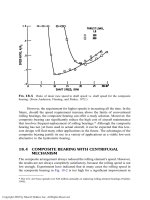
way, water promotes contact fatigue in rolling-element bearings. It is well known
that water penetration into the bearings is often a major problem in centrifugal
pumps; wherever it occurs, it causes an early bearing failure, particularly for
rolling-element bearings, which involve high fatigue stresses.
Rust inhibitors are oil additives that are absorbed on the surfaces of ferrous
alloys in preference to water, thus preventing corrosion. Also, metal deactivators
are additives that reduce nonferrous metal corrosion. Similar to rust inhibitors,
they are preferentially absorbed on the surface and are effective in protecting it

from corrosion. Examples of rust inhibitors are oil-soluble petroleum sulfonates
and calcium sulfonate, which can increase corrosion protection.
3.6.8 Antifoaming Additives
Foaming of liquid lubricants is undesirable because the bubbles deteriorate the
performance of hydrodynamic oil films in the bearing. In addition, foaming
adversely affects the oil supply of lubrication systems (it reduces the flow rate of
oil pumps). Also, the lubricant can overflow from its container (similar to the use
of liquid detergent without antifoaming additives in a washing machine). The
function of antifoaming additives is to increase the interfacial tension between the
gas and the lubricant. In this way, the bubbles collapse, allowing the gas to
escape.
Problems
3-1 Find the viscosity of the following three lubricants at 20

Cand
100

C:
a. SAE 30
b. SAE 10W-30
c. Polyalkylene glycol synthetic oil
Copyright 2003 by Marcel Dekker, Inc. All Rights Reserved.
List the three oils according to the sensitivity of viscosity to
temperature, based on the ratio of viscosity at 20

C to viscosity at
100

C.
3-2 Explain the advantages of synthetic oils in comparison to mineral oil.

Suggest an example application where there is a justification for using
synthetic oil of higher cost.
3-3 List five of the most widely used synthetic oils. What are the most
important characteristics of each of them?
3-4 Compare the advantages of using greases versus liquid lubricants.
Suggest two example applications where you would prefer to use
grease for lubrication and two examples where you would prefer to
use liquid lubricant. Justify your selection in each case.
3-5 a. Explain the process of oil degradation by oxidation.
b. List the factors that determine the oxidation rate.
c. List the various types of oxidation inhibitors.
Copyright 2003 by Marcel Dekker, Inc. All Rights Reserved.
4
Principles of Hydrodynamic
Lubrication
4.1 INTRODUCTION
A hydrodynamic plane-slider is shown in Fig. 1-2 and the widely used hydro-
dynamic journal bearing is shown in Fig. 1-3. Hydrodynamic lubrication is the
fluid dynamic effect that generates a lubrication fluid film that completely
separates the sliding surfaces. The fluid film is in a thin clearance between two
surfaces in relative motion. The hydrodynamic effect generates a hydrodynamic
pressure wave in the fluid film that results in load-carrying capacity, in the sense
that the fluid film has sufficient pressure to carry the external load on the bearing.
The pressure wave is generated by a wedge of viscous lubricant drawn into the
clearance between the two converging surfaces or by a squeeze-film action.
The thin clearance of a plane-slider and a journal bearing has the shape of a
thin converging wedge. The fluid adheres to the solid surfaces and is dragged into
the converging clearance. High shear stresses drag the fluid into the wedge due to
the motion of the solid surfaces. In turn, high pressure must build up in the fluid
film before the viscous fluid escapes through the thin clearance. The pressure

wave in the fluid film results in a load-carrying capacity that supports the external
load on the bearing. In this way, the hydrodynamic film can completely separate
the sliding surfaces, and, thus, wear of the sliding surfaces is prevented. Under
steady conditions, the hydrodynamic load capacity, W , of a bearing is equal to the
external load, F, on the bearing, but it is acting in the opposite direction. The
Copyright 2003 by Marcel Dekker, Inc. All Rights Reserved.
hydrodynamic theory of lubrication solves for the fluid velocity, pressure wave,
and resultant load capacity.
Experiments and hydrodynamic analysis indicated that the hydrodynamic
load capacity is proportional to the sliding speed and fluid viscosity. At the same
time, the load capacity dramatically increases for a thinner fluid film. However,
there is a practical limit to how much the bearing designer can reduce the film
thickness. A very thin fluid film is undesirable, particularly in machines with
vibrations. Whenever the hydrodynamic film becomes too thin, it results in
occasional contact of the surfaces, which results in severe wear. Picking the
optimum film-thickness is an important decision in the design process; it will be
discussed in the following chapters.
Tower (1880) conducted experiments and demonstrated for the first time
the existence of a pressure wave in a hydrodynamic journal bearing. Later,
Reynolds (1886) derived the classical theory of hydrodynamic lubrication. A
large volume of analytical and experimental research work in hydrodynamic
lubrication has subsequently followed the work of Reynolds. The classical theory
of Reynolds and his followers is based on several assumptions that were adopted
to simplify the mathematical derivations, most of which are still applied today.
Most of these assumptions are justified because they do not result in a significant
deviation from the actual conditions in the bearing. However, some other classical
assumptions are not realistic but were necessary to simplify the analysis. As in
other disciplines, the introduction of computers permitted complex hydrodynamic
lubrication problems to be solved by numerical analysis and have resulted in the
numerical solution of such problems under realistic conditions without having to

rely on certain inaccurate assumptions.
At the beginning of the twentieth century, only long hydrodynamic journal
bearings had been designed. The length was long in comparison to the diameter,
L > D; long-bearing theory of Reynolds is applicable to such bearings. Later,
however, the advantages of a short bearing were recognized. In modern machin-
ery, the bearings are usually short, L < D; short-bearing theory is applicable. The
advantage of a long bearing is its higher load capacity in comparison to a short
bearing. Moreover, the load capacity of a long bearing is even much higher per
unit of bearing area. In comparison, the most important advantages of a short
bearing that make it widely used are: (a) better cooling due to faster circulation of
lubricant; (b) less sensitivity to misalignment; and (c) a compact design.
Simplified models are commonly used in engineering to provide insight and
simple design tools. Hydrodynamic lubrication analysis is much simplified if the
bearing is assumed to be infinitely long or infinitely short. But for a finite-length
bearing, there is a three-dimensional flow that requires numerical solution by
computer. In order to simplify the analysis, long journal bearings, L > D, are
often solved as infinitely long bearings, while short bearings, L < D, are often
solved as infinitely short bearings.
Copyright 2003 by Marcel Dekker, Inc. All Rights Reserved.
4.2 ASSUMPTIONS OF HYDRODYNAMIC
LUBRICATION THEORY
The first assumption of hydrodynamic lubrication theory is that the fluid film flow
is laminar. The flow is laminar at low Reynolds number (Re). In fluid dynamics,
the Reynolds number is useful for estimating the ratio of the inertial and viscous
forces. For a fluid film flow, the expression for the Reynolds number is
Re ¼
Urh
m
¼
Uh

n
ð4-1Þ
Here, h is the average magnitude of the variable film thickness, r is the fluid
density, m is the fluid viscosity, and n is the kinematic viscosity. The transition
from laminar to turbulent flow in hydrodynamic lubrication initiates at about
Re ¼ 1000, and the flow becomes completely turbulent at about Re ¼ 1600. The
Reynolds number at the transition can be lower if the bearing surfaces are rough
or in the presence of vibrations. In practice, there are always some vibrations in
rotating machinery.
In most practical bearings, the Reynolds number is sufficiently low,
resulting in laminar fluid film flow. An example problem is included in Chapter
5, where Re is calculated for various practical cases. That example shows that in
certain unique applications, such as where water is used as a lubricant (in certain
centrifugal pumps or in boats), the Reynolds number is quite high, resulting in
turbulent fluid film flow.
Classical hydrodynamic theory is based on the assumption of a linear
relation between the fluid stress and the strain-rate. Fluids that demonstrate such a
linear relationship are referred to as Newtonian fluids (see Chapter 2). For most
lubricants, including mineral oils, synthetic lubricants, air, and water, a linear
relationship between the stress and the strain-rate components is a very close
approximation. In addition, liquid lubricants are considered to be incompressible.
That is, they have a negligible change of volume under the usual pressures in
hydrodynamic lubrication.
Differential equations are used for theoretical modeling in various disci-
plines. These equations are usually simplified under certain conditions by
disregarding terms of a relatively lower order of magnitude. Order analysis of
the various terms of an equation, under specific conditions, is required for
determining the most significant terms, which capture the most important effects.
A term in an equation can be disregarded and omitted if it is lower by one or
several orders of magnitude in comparison to other terms in the same equation.

Dimensionless analysis is a useful tool for determining the relative orders of
magnitude of the terms in an equation. For example, in fluid dynamics, the
Copyright 2003 by Marcel Dekker, Inc. All Rights Reserved.
dimensionless Reynolds number is a useful tool for estimating the ratio of inertial
and viscous forces.
In hydrodynamic lubrication, the fluid film is very thin, and in most
practical cases the Reynolds number is low. Therefore, the effect of the inertial
forces of the fluid (ma) as well as gravity forces (mg) are very small and can be
neglected in comparison to the dominant effect of the viscous stresses. This
assumption is applicable for most practical hydrodynamic bearings, except in
unique circumstances.
The fluid is assumed to be continuous, in the sense that there is continuity
(no sudden change in the form of a step function) in the fluid flow variables, such
as shear stresses and pressure distribution. In fact, there are always very small air
bubbles in the lubricant that cause discontinuity. However, this effect is usually
negligible, unless there is a massive fluid foaming or fluid cavitation (formation
of bubbles when the vapor pressure is higher than the fluid pressure). In general,
classical fluid dynamics is based on the continuity assumption. It is important for
mathematical derivations that all functions be continuous and differentiable, such
as stress, strain-rate, and pressure functions.
The following are the basic ten assumptions of classical hydrodynamic
lubrication theory. The first nine were investigated and found to be justified, in the
sense that they result in a negligible deviation from reality for most practical oil
bearings (except in some unique circumstances). The tenth assumption however,
has been introduced only for the purpose of simplifying the analysis.
Assumptions of classical hydrodynamic lubrication theory
1. The flow is laminar because the Reynolds number, Re,islow.
2. The fluid lubricant is continuous, Newtonian, and incompressible.
3. The fluid adheres to the solid surface at the boundary and there is no
fluid slip at the boundary; that is, the velocity of fluid at the solid

boundary is equal to that of the solid.
4. The velocity component, n, across the thin film (in the y direction) is
negligible in comparison to the other two velocity components, u and
w, in the x and z directions, as shown in Fig. 1-2.
5. Velocity gradients along the fluid film, in the x and z directions, are
small and negligible relative to the velocity gradients across the film
because the fluid film is thin, i.e., du=dy  du=dx and
dw=dy  dw=dz.
6. The effect of the curvature in a journal bearing can be ignored. The
film thickness, h, is very small in comparison to the radius of
curvature, R, so the effect of the curvature on the flow and pressure
distribution is relatively small and can be disregarded.
Copyright 2003 by Marcel Dekker, Inc. All Rights Reserved.
7. The pressure, p, across the film (in the y direction) is constant. In fact,
pressure variations in the y direction are very small and their effect is
negligible in the equations of motion.
8. The force of gravity on the fluid is negligible in comparison to the
viscous forces.
9. Effects of fluid inertia are negligible in comparison to the viscous
forces. In fluid dynamics, this assumption is usually justified for low-
Reynolds-number flow.
These nine assumptions are justified for most practical hydrodynamic
bearings. In contrast, the following additional tenth assumption has been
introduced only for simplification of the analysis.
10. The fluid viscosity, m, is constant.
It is well known that temperature varies along the hydrodynamic film,
resulting in a variable viscosity. However, in view of the significant simplification
of the analysis, most of the practical calculations are still based on the assumption
of a constant equivalent viscosity that is determined by the average fluid film
temperature. The last assumption can be applied in practice because it has already

been verified that reasonably accurate results can be obtained for regular
hydrodynamic bearings by considering an equivalent viscosity. The average
temperature is usually determined by averaging the temperature of the bearing
inlet and outlet lubricant. Various other methods have been suggested to calculate
the equivalent viscosity.
A further simplification of the analysis can be obtained for very long and
very short bearings. If a bearing is very long, the flow in the axial direction (z
direction) can be neglected, and the three-dimensional flow reduces to a much
simpler two-dimensional flow problem that can yield a closed form of analytical
solution.
A long journal bearing is where the bearing length is much larger than its
diameter, L  D, and a short journal bearing is where L  D.IfL  D, the
bearing is assumed to be infinitely long; if L  D, the bearing is assumed to be
infinitely short.
For a journal bearing whose length L and diameter D are of a similar order
of magnitude, the analysis is more complex. This three-dimensional flow analysis
is referred to as a finite-length bearing analysis. Computer-aided numerical
analysis is commonly applied to solve for the finite bearing. The results are
summarized in tables that are widely used for design purposes (see Chapter 8).
Copyright 2003 by Marcel Dekker, Inc. All Rights Reserved.
4.3 HYDRODYNAMIC LONG BEARING
The coordinates of a long hydrodynamic journal bearing are shown in Fig. 4-1.
The velocity components of the fluid flow, u, v, and w are in the x; y, and z
directions, respectively. A journal bearing is long if the bearing length, L, is much
larger than its diameter, D. A plane-slider (see Fig. 1-2) is long if the bearing
width, L, in the z direction is much larger than the length, B, in the x direction (the
direction of the sliding motion), or L  B.
In addition to the ten classical assumptions, there is an additional assump-
tion for a long bearing—it can be analyzed as an infinitely long bearing. The
pressure gradient in the z direction (axial direction) can be neglected in

comparison to the pressure gradient in the x direction (around the bearing).
The pressure is assumed to be constant along the z direction, resulting in two-
dimensional flow, w ¼ 0.
In fact, in actual long bearings there is a side flow from the bearing edge, in
the z direction, because the pressure inside the bearing is higher than the ambient
pressure. This side flow is referred to as an end effect. In addition to flow, there
are other end effects, such as capillary forces. But for a long bearing, these effects
are negligible in comparison to the constant pressure along the entire length.
4.4 DIFFERENTIAL EQUATION OF FLUID
MOTION
The following analysis is based on first principles. It does not use the Navier–
Stokes equations or the Reynolds equation and does not require in-depth
knowledge of fluid dynamics. The following self-contained derivation can help
in understanding the physical concepts of hydrodynamic lubrication.
An additional merit of a derivation that does not rely on the Navier–Stokes
equations is that it allows extending the theory to applications where the Navier–
Stokes equations do not apply. An example is lubrication with non-Newtonian
fluids, which cannot rely on the classical Navier–Stokes equations because they
FIG. 4-1 Coordinates of a long journal bearing.
Copyright 2003 by Marcel Dekker, Inc. All Rights Reserved.
assume the fluid is Newtonian. Since the following analysis is based on first
principles, a similar derivation can be applied to non-Newtonian fluids (see
Chapter 19).
The following hydrodynamic lubrication analysis includes a derivation of
the differential equation of fluid motion and a solution for the flow and pressure
distribution inside a fluid film. The boundary conditions of the velocity and the
conservation of mass (or the equivalent conservation of volume for an incom-
pressible flow) are considered for this derivation.
The equation of the fluid motion is derived by considering the balance of
forces acting on a small, infinitesimal fluid element having the shape of a

rectangular parallelogram of dimensions dx and dy, as shown in Fig. 4-2. This
elementary fluid element inside the fluid film is shown in Fig. 1-2. The derivation
is for a two-dimensional flow in the x and y directions. In an infinitely long
bearing, there is no flow or pressure gradient in the z direction. Therefore, the
third dimension of the parallelogram (in the z direction) is of unit length (1).
The pressure in the x direction and the shear stress, t, in the y direction are
shown in Fig. 4-2. The stresses are subject to continuous variations. A relation
between the pressure and shear-stress gradients is derived from the balance of
forces on the fluid element. The forces are the product of stresses, or pressures,
and the corresponding areas. The fluid inertial force (ma) is very small and is
therefore neglected in the classical hydrodynamic theory (see assumptions listed
earlier), allowing the derivation of the following force equilibrium equation in a
similar way to a static problem:
ðt þ dtÞdx 1 t dx 1 ¼ðp þ dpÞdy 1 ¼ pdy1 ð4-2Þ
Equation (4-2) reduces to
dt dx ¼ dp dy ð4-3Þ
FIG. 4-2 Balance of forces on an infinitesimal fluid element.
Copyright 2003 by Marcel Dekker, Inc. All Rights Reserved.
After substituting the full differential expression dt ¼ð@t=@yÞdy in Eq. (4-3) and
substituting the equation t ¼ m ð@u=@yÞ for the shear stress, Eq. (4-3) takes the
form of the following differential equation:
dp
dx
¼ m
@
2
u
@y
2
ð4-4Þ

A partial derivative is used because the velocity, u, is a function of x and y.
Equation (4-4), is referred to as the equation of fluid motion, because it can be
solved for the velocity distribution, u, in a thin fluid film of a hydrodynamic
bearing.
Comment. In fact, it is shown in Chapter 5 that the complete equation for
the shear stress is t ¼ mðdu=dy þ dv=dxÞ. However, according to our assump-
tions, the second term is very small and is neglected in this derivation.
4.5 FLOW IN A LONG BEARING
The following simple solution is limited to a fluid film of steady geometry. It
means that the geometry of the fluid film does not vary with time relative to the
coordinate system, and it does not apply to time-dependent fluid film geometry
such as a bearing under dynamic load. A more universal approach is possible by
using the Reynolds equation (see Chapter 6). The Reynolds equation applies to
all fluid films, including time-dependent fluid film geometry.
Example Problems 4-1
Journal Bearing
In Fig. 4-1, a journal bearing is shown in which the bearing is stationary and the
journal turns around a stationary center. Derive the equations for the fluid velocity
and pressure gradient.
The variable film thickness is due to the journal eccentricity. In hydro-
dynamic bearings, h ¼ hðxÞ is the variable film thickness around the bearing. The
coordinate system is attached to the stationary bearing, and the journal surface
has a constant velocity, U ¼ oR, in the x direction.
Solution
The coordinate x is along the bearing surface curvature. According to the
assumptions, the curvature is disregarded and the flow is solved as if the
boundaries were a straight line.
Equation (4-4) can be solved for the velocity distribution, u ¼ uðx; yÞ.
Following the assumptions, variations of the pressure in the y direction are
negligible (Assumption 6), and the pressure is taken as a constant across the film

Copyright 2003 by Marcel Dekker, Inc. All Rights Reserved.
thickness because the fluid film is thin. Therefore, in two-dimensional flow of a
long bearing, the pressure is a function of x only. In order to simplify the solution
for the velocity, u, the following substitution is made in Eq. (4-4):
2mðxÞ¼
1
m
dp
dx
ð4-5Þ
where mðxÞ is an unknown function of x that must be solved in order to find the
pressure distribution. Equation 4-4 becomes
@u
2
@y
2
¼ 2mðxÞð4-6Þ
Integrating Eq. (4-6) twice yields the following expression for the velocity
distribution, u, across the fluid film (n and k are integration constants):
u ¼ my
2
þ ny þk ð4-7Þ
Here, m, n, and k are three unknowns that are functions of x only. Three equations
are required to solve for these three unknowns. Two equations are obtained from
the two boundary conditions of the flow at the solid surfaces, and the third
equation is derived from the continuity condition, which is equivalent to the
conservation of mass of the fluid (or conservation of volume for incompressible
flow).
The fluid adheres to the solid wall (no slip condition), and the fluid velocity
at the boundaries is equal to that of the solid surface. In a journal bearing having a

stationary bearing and a rotating journal at surface speed U ¼ oR (see Fig. 4-1),
the boundary conditions are
at y ¼ 0: u ¼ 0
at y ¼ hðxÞ: u ¼ U cos a  U
ð4-8Þ
The slope between the tangential velocity U and the x direction is very small;
therefore, cos a  1, and we can assume that at y ¼ hðxÞ, u  U.
The third equation, which is required for the three unknowns, m; n, and k,is
obtained from considerations of conservation of mass. For an infinitely long
bearing, there is no flow in the axial direction, z; therefore, the amount of mass
flow through each cross section of the fluid film is constant (the cross-sectional
plane is normal to the x direction). Since the fluid is incompressible, the volume
flow rate is also constant at any cross section. The constant-volume flow rate, q,
per unit of bearing length is obtained by integration of the velocity component, u,
along the film thickness, as follows:
q ¼
ð
h
0
udy¼ constant ð4-9Þ
Copyright 2003 by Marcel Dekker, Inc. All Rights Reserved.
Equation (4-9) is applicable only for a steady fluid film geometry that does not
vary with time.
The pressure wave around the journal bearing is shown in Fig. 1-3. At the
peak of the pressure wave, dp=dx ¼ 0, and the velocity distribution, u ¼ uðyÞ,at
that point is linear according to Eq. (4-4). The linear velocity distribution in a
simple shear flow (in the absence of pressure gradient) is shown in Fig. 4-3. If the
film thickness at the peak pressure point is h ¼ h
0
, the flow rate, q, per unit length

is equal to the area of the velocity distribution triangle:
q ¼
Uh
0
2
ð4-10Þ
The two boundary conditions of the velocity as well as the conservation of mass
condition form the following three equations, which can be solved for m, n and k:
0 ¼ m0
2
þ n0 þk ) k ¼ 0
U ¼ mh
2
þ nh
Uh
0
2
¼
ð
h
0
ðmy
2
þ nyÞ dy
ð4-11Þ
After solving for m, n, and k and substituting these values into Eq. (4-7), the
following equation for the velocity distribution is obtained:
u ¼ 3U
1
h

2

h
0
h
3

y
2
þ U
3h
0
h
2

2
h

y ð4-12Þ
FIG. 4-3 Linear velocity distribution for a simple shear flow (no pressure gradient).
Copyright 2003 by Marcel Dekker, Inc. All Rights Reserved.
From the value of m, the expression for the pressure gradient, dp=dx, is solved
[see Eq. (4-5)]:
dp
dx
¼ 6Um
h  h
0
h
3

ð4-13Þ
Equation (4-13) still contains an unknown constant, h
0
, which is the film
thickness at the peak pressure point. This will be solved from additional
information about the pressure wave. Equation (4-13) can be integrated for the
pressure wave.
Example Problem 4-2
Inclined Plane Slider
As discussed earlier, a steady-fluid-film geometry (relative to the coordinates)
must be selected for a simple derivation of the pressure gradient. The second
example is of an inclined plane-slider having a configuration as shown in Fig. 4-
4. This example is of a converging viscous wedge similar to that of a journal
bearing; however, the lower part is moving in the x direction and the upper plane
is stationary while the coordinates are stationary. This bearing configuration is
selected because the geometry of the clearance (and fluid film) does not vary with
time relative to the coordinate system.
Find the velocity distribution and the equation for the pressure gradient in
the inclined plane-slider shown in Fig 4-4.
Solution
In this case, the boundary conditions are:
at y ¼ 0: u ¼ U
at y ¼ hðxÞ: u ¼ 0
In this example, the lower boundary is moving and the upper part is stationary.
The coordinates are stationary, and the geometry of the fluid film does not vary
FIG. 4-4 Inclined plane-slider (converging flow in the x direction).
Copyright 2003 by Marcel Dekker, Inc. All Rights Reserved.
relative to the coordinates. In this case, the flow rate is constant, in a similar way
to that of a journal bearing. This flow rate is equal to the area of the velocity
distribution triangle at the point of peak pressure, where the clearance thickness is

h
0
. The equation for the constant flow rate is
q ¼
ð
h
0
udy¼
h
0
U
2
The two boundary conditions of the velocity and the constant flow-rate condition
form the three equations for solving for m, n, and k:
U ¼ m0
2
þ n0 þk ) k ¼ U
0 ¼ mh
2
þ nh þU
Uh
0
2
¼
ð
h
0
ðmy
2
þ ny þ U Þdy

After solving for m, n, and k and substituting these values into Eq. (4-7), the
following equation for the velocity distribution is obtained:
u ¼ 3U
1
h
2

h
0
h
3

y
2
þ U
3h
0
h
2

4
h

y þ U
From the value of m, an identical expression to Eq. (4-13) for the pressure
gradient, dp=dx, is obtained for @h=@x < 0 (a converging slope in the x direction):
dp
dx
¼ 6Um
h  h

0
h
3
for
@h
@x
< 0 ðnegative slopeÞ
This equation applies to a converging wedge where the coordinate x is in the
direction of a converging clearance. It means that the clearance reduces along x as
shown in Fig. 4-4.
In a converging clearance near x ¼ 0, the clearance slope is negative,
@h=@x < 0. This means that the pressure increases near x ¼ 0. At that point,
h > h
0
, resulting in dp=dx > 0.
If we reverse the direction of the coordinate x, the expression for the
pressure gradient would have an opposite sign:
dp
dx
¼ 6Um
h
0
 h
h
3
for
@h
@x
> 0 ðpositive slopeÞ
This equation applies to a plane-slider, as shown in Fig 4-5, where the coordinate

x is in the direction of increasing clearance. The unknown constant, h
0
, will be
determined from the boundary conditions of the pressure wave.
Copyright 2003 by Marcel Dekker, Inc. All Rights Reserved.
tions has been a challenge in the past. However, the use of computers makes
numerical integration a relatively easy task.
An inclined plane slider is shown in Fig. 4-5, where the inclination angle is
a. The fluid film is equivalent to that in Fig. 4-4, although the x is in the opposite
direction, @h=@x > 0, and the pressure wave is
p ¼ 6mU
ð
x
x
1
h
0
 h
h
3
dx ð4-14bÞ
In order to have concise equations, the slope of the plane-slider is
substituted by a ¼ tan a, and the variable film thickness is given by the function
hðxÞ¼ax ð4-15Þ
Here, x is measured from the point of intersection of the plane-slider and the
bearing surface. The minimum and maximum film thicknesses are h
1
and h
2
,

respectively, as shown in Fig. 4-5.
In order to solve the pressure distribution in any converging fluid film, Eq.
(4-14) is integrated after substituting the value of h according to Eq. (4-15). After
integration, there are two unknowns: the constant h
0
in Eq. (4-10) and the
constant of integration, p
o
. The two unknown constants are solved for the two
boundary conditions of the pressure wave. At each end of the inclined plane, the
pressure is equal to the ambient (atmospheric) pressure, p ¼ 0. The boundary
conditions are:
at h ¼ h
1
: p ¼ 0
at h ¼ h
2
: p ¼ 0
ð4-16Þ
The solution can be analytically performed in closed form or by numerical
integration (see Appendix B). The numerical integration involves iterations to
find h
0
. Hydrodynamic lubrication equations require frequent use of computer
programming to perform the trial-and-error iterations. An example of a numerical
integration is shown in Example Problem 4-4.
Analytical Solution. For an infinitely long plane-slider, L  B, analytical
integration results in the following pressure wave along the x direction (between
x ¼ h
1

=a and x ¼ h
2
=a):
p ¼
6mU
a
3
ðh
1
 axÞðax h
2
Þ
ðh
1
þ h
2
Þx
2
ð4-17Þ
At the boundaries h ¼ h
1
and h ¼ h
2
, the pressure is zero (atmospheric pressure).
Copyright 2003 by Marcel Dekker, Inc. All Rights Reserved.
4.7 PLANE-SLIDER LOAD CAPACITY
Once the pressure wave is solved, it is possible to integrate it again to solve for the
bearing load capacity, W . For a plane-slider, the integration for the load capacity
is according to the following equation:
W ¼ L

ð
x
2
x
1
pdx ð4-18Þ
The foregoing integration of the pressure wave can be derived analytically, in
closed form. However, in many cases, the derivation of an analytical solution is
too complex, and a computer program can perform a numerical integration. It is
beneficial for the reader to solve this problem numerically, and writing a small
computer program for this purpose is recommended.
An analytical solution for the load capacity is obtained by substituting the
pressure in Eq. (4-17) into Eq. (4-18) and integrating in the boundaries between
x
1
¼ h
1
=a and x
2
¼ h
2
=a. The final analytical expression for the load capacity in
a plane-slider is as follows:
W ¼
6mULB
2
h
2
2
1

b  1

2
ln b 
2ðb  1Þ
b þ 1
!
ð4-19Þ
where b is the ratio of the maximum and minimum film thickness, h
2
=h
1
.A
similar derivation can be followed for nonflat sliders, such as in the case of a
slider having a parabolic surface in Problem 4-2, at the end of this chapter.
4.8 VISCOUS FRICTION FORCE IN A PLANE-
SLIDER
The friction force, F
f
, is obtained by integrating the shear stress, t over any cross-
sectional area along the fluid film. For convenience, a cross section is selected
along the bearing stationary wall, y ¼ 0. The shear stress at the wall, t
w
,aty ¼ 0
can be obtained via the following equation:
t
w
¼ m
du
dy

j
ðy¼0Þ
ð4-20Þ
The velocity distribution can be substituted from Eq. (4-12), and after differ-
entiation of the velocity function according to Eq. (4-20), the shear stress at the
wall, y ¼ 0, is given by
t
w
¼ mU
3h
0
h
2

2
h

ð4-21Þ
Copyright 2003 by Marcel Dekker, Inc. All Rights Reserved.
The friction force, F
f
, for a long plane-slider is obtained by integration of the
shear stress, as follows:
F
f
¼ L
ð
x
2
x

1
t dx ð4-22Þ
4.8.1 Friction Coe⁄cient
The bearing friction coefficient, f , is defined as the ratio of the friction force to
the bearing load capacity:
f ¼
F
f
W
ð4-23Þ
An important objective of a bearing design is to minimize the friction coefficient.
The friction coefficient is usually lower with a thinner minimum film thickness,
h
n
(in a plane-slider, h
n
¼ h
1
). However, if the minimum film thickness is too low,
it involves the risk of severe wear between the surfaces. Therefore, the design
involves a compromise between a low-friction requirement and a risk of severe
wear. Determination of the desired minimum film thickness, h
n
, requires careful
consideration. It depends on the surface finish of the sliding surfaces and the level
of vibrations and disturbances in the machine. This part of the design process is
discussed in the following chapters.
4.9 FLOW BETWEEN TWO PARALLEL PLATES
Example Problem 4-3
Derive the equation of the pressure gradient in a unidirectional flow inside a thin

clearance between two stationary parallel plates as shown in Fig. 4-6. The flow is
parallel, in the x direction only. The constant clearance between the plates is h
0
,
and the rate of flow is Q, and the x axis is along the center of the clearance.
FIG. 4-6 Flow between two parallel plates.
Copyright 2003 by Marcel Dekker, Inc. All Rights Reserved.
Solution
In a similar way to the solution for hydrodynamic bearing, the parallel flow in the
x direction is derived from Eq. (4-4), repeated here as Eq. (4-24):
dp
dx
¼ m
@
2
u
@y
2
ð4-24Þ
This equation can be rewritten as
@u
2
@y
2
¼
1 dp
m dx
ð4-25Þ
The velocity profile is solved by a double integration. Integrating Eq. (4-25) twice
yields the expression for the velocity u:

u ¼
1
2m
dp
dx
y
2
þ ny þk ð4-26Þ
Here, n and k are integration constants obtained from the two boundary
conditions of the flow at the solid surfaces (no-slip condition).
The boundary conditions at the wall of the two plates are:
at y ¼
h
0
2
: u ¼ 0 ð4-27Þ
The flow is symmetrical, and the solution for n and k is
n ¼ 0; k ¼m
h
0
2

2
ð4-28Þ
The flow equation becomes
u ¼
1
2m
dp
dx

y
2

h
2
4

ð4-29Þ
The parabolic velocity distribution is shown in Fig. 4-6. The pressure gradient is
obtained from the conservation of mass. For a parallel flow, there is no flow in the
z direction. For convenience, the y coordinate is measured from the center of the
clearance. The constant-volume flow rate, Q, is obtained by integrating the
velocity component, u, along the film thickness, as follows:
Q ¼ 2L
ð
h=2
0
udy ð4-30Þ
Copyright 2003 by Marcel Dekker, Inc. All Rights Reserved.