Advanced Vehicle Technology Episode 2 Part 2 potx

6.2 The need for constant velocity joints
Universal joints are necessary to transmit torque
and rotational motion from one shaft to another
when their axes do not align but intersect at some
point. This means that both shafts are inclined to
each other by some angle which under working
conditions may be constantly varying.
Universal joints are incorporated as part of a
vehicle's transmission drive to enable power to be
transferred from a sprung gearbox or final drive to
the unsprung axle or road wheel stub shaft.
There are three basic drive applications for the
universal joint:
1 propellor shaft end joints between longitudinally
front mounted gearbox and rear final drive axle,
2 rear axle drive shaft end joints between the
sprung final drive and the unsprung rear wheel
stub axle,
3 front axle drive shaft end joints between the
sprung front mounted final drive and the
unsprung front wheel steered stub axle.
Universal joints used for longitudinally mounted
propellor shafts and transverse rear mounted drive
shafts have movement only in the vertical plane.
The front outer drive shaft universal joint has to
cope with movement in both the vertical and hori-
zontal plane; it must accommodate both vertical
suspension deflection and the swivel pin angular
movement to steer the front road wheels.
The compounding of angular working move-
ment of the outer drive shaft steering joint in two

planes imposes abnormally large and varying
working angles at the same time as torque is being
transmitted to the stub axle. Because of the severe
working conditions these joints are subjected to
special universal joints known as constant velocity
joints. These have been designed and developed to
eliminate torque and speed fluctuations and to
operate reliability with very little noise and wear
and to have a long life expectancy.
6.2.1 Hooke's universal joint (Figs 6.29 and 6.30)
The Hooke's universal joint comprises two yoke
arm members, each pair of arms being positioned
at right angles to the other and linked together by
an intermediate cross-pin member known as the
spider. When assembled, pairs of cross-pin legs
are supported in needle roller caps mounted in
each yoke arm, this then permits each yoke mem-
ber to swing at right angles to the other.
Because pairs of yoke arms from one member are
situated in between arms of the other member, there
will be four extreme positions for every revolution
when the angular movement is taken entirely by
only half of the joint. As a result, the spider cross-
pins tilt back and forth between these extremes so
that if the drive shaft speed is steady throughout
every complete turn, the drive shaft will accelerate
and decelerate twice during one revolution, the mag-
nitude of speed variation becoming larger as the
drive to driven shaft angularity is increased.
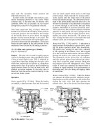
Hooke's joint speed fluctuation may be better

understood by considering Fig. 6.29. This shows
the drive shaft horizontal and the driven shaft
inclined downward. At zero degree movement the
input yoke cross-pin axis is horizontal when the
drive shaft and the output yoke cross-pin axis are
vertical. In this position the output shaft is at a
minimum. Conversely, when the input shaft has
rotated a further 90

, the input and output yokes
and cross-pins will be in the vertical and horizontal
position respectively. This produces a maximum
output shaft speed. A further quarter of a turn will
move the joint to an identical position as the initial
position so that the output speed will be again at a
minimum. Thus it can be seen that the cycle of
events repeat themselves every half revolution.
Table 6.2 shows how the magnitude of the speed
fluctuation varies with the angularity of the drive
to driven shafts.
The consequences of only having a single
Hooke's universal joint in the transmission line
can be appreciated if the universal joint is con-
sidered as the link between the rotating engine
and the vehicle in motion, moving steadily on the
road. Imagine the engine's revolving inertia masses
rotating at some constant speed and the vehicle
itself travelling along uniformly. Any cyclic speed
variation caused by the angularity of the input and
output shafts will produce a correspondingly peri-

odic driving torque fluctuation. As a result of this
torque variation, there will be a tendency to wind
and unwind the drive in proportion to the working
angle of the joint, thereby imposing severe stresses
upon the transmission system. This has been found
to produce uneven wear on the driving tyres.
To eliminate torsional shaft cyclic peak stresses
and wind-up, universal joints which rotate uni-
formly during each revolution become a necessity.
Table 6.2 Variation of shaft angle with speed fluctuation
Shaft angle (deg) 5 10 15 20 25 30 35 40
% speed fluctuation 0.8 3.0 6.9 12.4 19.7 28.9 40.16 54
212
6.2.2 Hooke's joint cyclic speed variation due to
drive to driven shaft inclination (Fig. 6.30)
Consider the Hooke's joint shown in Fig. 6.30(a)
with the input and output yokes in the horizontal
and vertical position respectively and the output
shaft inclined  degrees to the input shaft.
Let !
i
=input shaft angular velocity (rad/sec)
!
o
=output shaft angular velocity (rad/sec)
Â=shaft inclination (deg)
R=pitch circle joint radius (mm)
Then
Linear velocity of point (p)  !
i

y
and
Linear velocity of point (p)  !
o
R.
Since these velocities are equal,
!
o
R  !
i
y
; !
o
 !
i
y
R
but
y
R
 cos Â:
Thus !
o
 !
i
cos Â
but !
i

2

60
N
i
:
So
2
60
N
o

2
60
N
i
cos Â
Hence N
o
N
i
cos  (this being a minimum) (1):
If now the joint is rotated a quarter of a revolu-
tion (Fig. 6.30(b)) the input and output yoke posi-
tions will be vertical and horizontal respectively.
Then
Linear velocity of point (p)  !
o
y
also
Linear velocity of point (p)  !
i

R:
Since these velocities are equal,
!
o
y  !
i
R
!
o
 !
i
R
y
but
R
y

1
cos Â
:
Fig. 6.29 Hooke's joint cycle of speed fluctuation for 30

shaft angularity
213
Thus !
o

!
i
cos Â

2
60
N
o

2
60
N
i
cos Â
N
o

N
i
cos Â
(this being a maximum) (2)
Note
1Wheny  R the angular instantaneous velocities
will be equal.
2Wheny is smaller than R, the output instanta-
neous velocity will be less than the output.
3Wheny is larger than R, the output instanta-
neous velocity will be greater than the input.
Example 1 A Hooke's universal joint connects two
shafts which are inclined at 30

to each other. If the
driving shaft speed is 500 rev/min, determine the
maximum and minimum speeds of the driven shaft.

Minimum speed N
o
 N
i
cos 30
 500 Â0:866
 433 (rev=min)
Maximum speed N
o

N
i
cos 30

500
0:866
 577 (rev=min)
Example 2 A Hooke's universal joint connects
two shafts which are inclined at some angle. If the
input and output joint speeds are 500 and 450 rev/
min respectively, find the angle of inclination of the
output shaft.
N
o
 N
i
cos Â
cos  
N
o

N
i
Hence cos  
450
500
 0:9
Therefore   25850
H
6.2.3 Constant velocity joints
Constant velocity joints imply that when two shafts
are inclined at some angle to one another and they
are coupled together by some sort of joint, then a
uniform input speed transmitted to the output shaft
produces the same angular output speed throughout
one revolution. There will be no angular accelera-
tion and deceleration as the shafts rotate.
6.2.4 Double Hooke's type constant velocity joint
(Figs 6.31 and 6.32)
One approach to achieve very near constant velocity
characteristics is obtained by placing two Hooke's
type joint yoke members back to back with their
yoke arms in line with one another (Fig. 6.31).
When assembled, both pairs of outer yoke arms will
be at right angles to the arms of the central double
yoke member. Treating this double joint combina-
tion in two stages, the first stage hinges the drive yoke
and driven central double yoke together, whereas the
second stage links the central double yoke (now drive
member) to the driven final output yoke. Therefore
the second stage drive half of the central double yoke

is positioned a quarter of a revolution out of phase
with the first stage drive yoke (Fig. 6.32).
Consequently when the input and output shafts
are inclined to each other and the first stage driven
central double yoke is speeding up, the second
stage driven output yoke will be slowing down.
Conversely when the first stage driven member is
reducing speed the second stage driven member
increases its speed; the speed lost or gained by one
half of the joint will equal that gained or lost by the
second half of the joint respectively. There will
therefore be no cyclic speed fluctuation between
input and output shafts during rotation.
An additional essential feature of this double
joint is a centring device (Fig. 6.31) normally of the
ball and socket spring loaded type. Its function is to
maintain equal angularity of both the input and
Fig. 6.30 (a and b) Hooke's joint geometry
214
output shafts relative to the central double yoke
member. This is a difficult task due to the high end
loads imposed on the sliding splined joint of the drive
shaft when repeated suspension deflection and large
drive torques are being transmitted simultaneously.
However, the accuracy of centralizing the double
yokes is not critical at the normal relatively low
drive shaft speeds.
This double Hooke's joint is particularly suitable
for heavy duty rigid front wheel drive live axle
vehicles where large lock-to-lock wheel swivel is

necessary. A major limitation with this type of
joint is its relatively large size for its torque trans-
mitting capacity.
6.2.5 Birfield joint based on the Rzeppa Principle
(Fig. 6.33)
Alfred Hans Rzeppa (pronounced sheppa), a Ford
engineer in 1926, invented one of the first practical
Fig. 6.31 Double Hooke's type constant velocity joint
Fig. 6.32 Double Hooke's type joint shown in two positions 90

out of phase
215
constant velocity joints which was able to transmit
torque over a wide range of angles without there
being any variation in the rotary motion of the
output shafts. An improved version was patented
by Rzeppa in 1935. This joint used six balls as
intermediate members which where kept at all
times in a plane which bisects the angle between
the input and output shafts (Fig. 6.33). This early
design of a constant velocity joint incorporated
a controlled guide ball cage which maintained the
balls in the bisecting plane (referred to as the med-
ian plane) by means of a pivoting control strut
which swivelled the cage at an angle of exactly
half that made between the driving and driven
shafts. This control strut was located in the centre
of the enclosed end of the outer cup member, both
ball ends of the strut being located in a recess and
socket formed in the adjacent ends of the driving

and driven members of the joint respectively. A
large spherical waist approximately midway along
the strut aligned with a hole made in the centre of
the cage. Any angular inclination of the two shafts
at any instant deflected the strut which in turn
proportionally swivelled the control ball cage at
half the relative angular movement of both shafts.
This method of cage control tended to jam and
suffered from mechanical wear.
Joint construction (Fig. 6.34) The Birfield joint,
based on the Rzeppa principle and manufactured
by Hardy Spicer Limited, has further developed and
improved the joint's performance by generating
converging ball tracks which do not rely on a con-
trolled ball cage to maintain the intermediate ball
members on the median plane (Fig. 6.34(b)). This
Fig. 6.33 Early Rzeppa constant velocity joint
216
Fig. 6.34 (a±c) Birfield Rzeppa type constant velocity joint
217
joint has an inner (ball) input member driving an
outer (cup) member. Torque is transmitted from the
input to the output member again by six intermedi-
ate ball members which fit into curved track grooves
formed in both the cup and spherical members.
Articulation of the joint is made possible by the
balls rolling inbetween the inner and outer pairs of
curved grooves.
Ball track convergence (Figs 6.34 and 6.35) Con-
stant velocity conditions are achieved if the points

of contact of both halves of the joint lie in a plane
which bisects the driving and driven shaft angle,
this being known as the median plane (Fig.
6.34(b)). These conditions are fulfilled by having
an intermediate member formed by a ring of six
balls which are kept in the median plane by the
shape of the curved ball tracks generated in both
the input and output joint members.
To obtain a suitable track curvature in both
half, inner and outer members so that a controlled
movement of the intermediate balls is achieved, the
tracks (grooves) are generated on semicircles. The
centres are on either side of the joint's geometric
centre by an equal amount (Figs 6.34(a) and 6.35).
The outer half cup member of the joint has the
centre of the semicircle tracks offset from the centre
of the joint along the centre axis towards the open
mouth of the cup member, whilst the inner half
spherical member has the centre of the semicircle
track offset an equal amount in the opposite direc-
tion towards the closed end of the joint (Fig. 6.35).
When the inner member is aligned inside the
outer one, the six matching pairs of tracks form
grooved tunnels in which the balls are sandwiched.
The innerand outertrack arc offsetcentre from the
geometric joint centre are so chosen to give an angle
of convergence (Fig. 6.35) marginally largerthan 11

,
which is the minimum amount necessary to positively

guide and keep the balls on the median plane over the
entire angular inclination movement of the joint.
Track groove profile (Fig. 6.36) The ball tracks in
the inner and outer members are not a single semi-
circle arc having one centre of curvature but
instead are slightly elliptical in section, having
effectively two centres of curvature (Fig. 6.36).
The radius of curvature of the tracks on each side
of the ball at the four pressure angle contact points
is larger than the ball radius and is so chosen so
that track contact occurs well within the arc
grooves, so that groove edge overloading is elimi-
nated. At the same time the ball contact load is
taken about one third below and above the top
and bottom ball tips so that compressive loading
of the balls is considerably reduced. The pressure
angle will be equal in the inner and outer tracks and
therefore the balls are all under pure compression
at all times which raises the limiting stress and
therefore loading capacity of the balls.
The ratio of track curvature radius to the ball
radius, known as the conformity ratio, is selected so
that a 45

pressure angle point contact is achieved,
which has proven to be effective and durable in
transmitting the torque from the driving to the
driven half members of the joint (Fig. 6.36).
As with any ball drive, there is a certain amount of
roll and slide as the balls move under load to and fro

along their respective tracks. By having a pressure
angle of 45

, the roll to sliding ratio is roughly 4:1.
Fig. 6.35 Birfield Rzeppa type joint showing ball track convergence
218
This is sufficient to minimize the contact friction
during any angular movement of the joint.
Ball cage (Fig. 6.34(b and c)) Both the inner drive
and outer driven members of the joint have spherical
external and internal surfaces respectively. Likewise,
the six ball intermediate members of this joint are
positioned in their respective tracks by a cage which
has the same centre of arc curvature as the input and
output members (Fig. 6.34(c)). The cage takes up
the space between the spherical surfaces of both
male inner and female outer members. It provides
the central pivot alignment for the two halves of the
joint when the input and output shafts are inclined
to each other (Fig. 6.34(b)).
Although the individual balls are theoretically
guided by the grooved tracks formed on the surfaces
of the inner and outer members, the overall align-
ment of all the balls on the median plane is provided
by the cage. Thus if one ball or more tends not to
position itself or themselves on the bisecting plane
between the two sets of grooves, the cage will auto-
matically nudge the balls into alignment.
Mechanical efficiency The efficiency of these
joints is high, ranging from 100% when the joint

working angle is zero to about 95% with a 45

joint
working angle. Losses are caused mainly by internal
friction between the balls and their respective
tracks, which is affected by ball load, speed and
working angle and by the viscous drag of the lubri-
cant, the latter being dependent to some extent by
the properties of the lubricant chosen.
Fault diagnoses Symptoms of front wheel drive
constant velocity joint wear or damage can be nar-
rowed down by turning the steering to full lock and
driving round in a circle. If the steering or trans-
mission now shows signs of excessive vibration or
clunking and ticking noises can be heard coming
from the drive wheels, further investigation of the
front wheel joints should be made. Split rubber
gaiters protecting the constant velocity joints can
considerably shorten the life of a joint due to expo-
sure to the weather and abrasive grit finding its way
into the joint mechanism.
6.2.6 Pot type constant velocity joint (Fig. 6.37)
This joint manufactured by both the Birfield and
Bendix companies has been designed to provide a
solution to the problem of transmitting torque with
varying angularity of the shafts at the same time as
accommodating axial movement.
There are four basic parts to this joint which
make it possible to have both constant velocity
characteristics and to provide axial plunge so that

the effective drive shaft length is able to vary as the
angularity alters (Fig. 6.37):
Fig. 6.36 Birfield joint rack groove profile
219
1 A pot input member which is of cylindrical shape
forms an integral part of the final drive stub shaft
and inside this pot are ground six parallel ball
grooves.
2 A spherical (ball) output member is attached by
splines to the drive shaft and ground on the
external surface of this sphere are six matching
straight tracked ball grooves.
3 Transmitting the drive from the input to the out-
put members are six intermediate balls which are
lodged between the internal and external grooves
of both pot and sphere.
4 A semispherical steel cage positions the balls on
a common plane and acts as the mechanism for
automatically bisecting the angle between the
drive and driven shafts (Fig. 6.38).
It is claimed that with straight cut internal and
external ball grooves and a spherical ball cage
which is positioned over the spherical (ball) output
member that a truly homokinetic (bisecting) plane
is achieved at all times. The joint is designed to
have a maximum operating angularity of 22

,44

including the angle, which makes it suitable for

independent suspension inner drive shaft joints.
6.2.7 Carl Weiss constant velocity joint
(Figs 6.38 and 6.40)
A successful constant velocity joint was initially
invented by Carl W. Weiss of New York, USA,
and was patented in 1925. The Bendix Products
Corporation then adopted the Weiss constant vel-
ocity principle, developed it and now manufacture
this design of joint (Fig. 6.38).
Joint construction and description With this type
of time constant velocity joint, double prong (arm)
yokes are mounted on the ends of the two shafts
transmitting the drive (Fig. 6.37). Ground inside
each prong member are four either curved or
straight ball track grooves (Fig. 6.39). Each yoke
arm of one member is assembled inbetween the
prong of the other member and four balls located
in adjacent grooved tracks transmit the drive from
one yoke member to the other. The intersection of
each matching pair of grooves maintains the balls
in a bisecting plane created between the two shafts,
even when one shaft is inclined to the other (Fig.
6.40). Depending upon application, some joint
models have a fifth centralizing ball inbetween the
two yokes while the other versions, usually with
straight ball tracks, do not have the central ball so
that the joint can accommodate a degree of axial
plunge, especially if, as is claimed, the balls roll
rather than slide.
Carl Weiss constant velocity principle (Fig. 6.41)

Consider the geometric construction of the
upper half of the joint (Fig. 6.41) with ball track
Fig. 6.37 Birfield Rzeppa pot type joint
220
curvatures on the left and right hand yokes to be
represented by circular arcs with radii (r) and cen-
tres of curvature L and R on their respective shaft
axes when both shafts are in line. The centre of the
joint is marked by point O and the intersection of
both the ball track arc centres occurs at point P.
Triangle L O P equals triangle R O P with sides L P
and R P being equal to the radius of curvature. The
offset of the centres of track curvature from the
joint centre are L O and R O, therefore sides L P
and R P are also equal. Now, angles L O P and
R O P are two right angles and their sum of
90

 90

is equal to the angle L O R, that is 180

,
so that point P lies on a perpendicular plane which
intersects the centre of the joint. This plane is
known as the median or homokinetic plane.
If the right hand shaft is now swivelled to a work-
ing angle its new centre of track curvature will be R
H
and the intersection point of both yoke ball track

curvatures is now P
H
(Fig. 6.41). Therefore triangle
LOP
H
andROP
H
are equal because both share the
same bisecting plane of the left and right hand
shafts. Thus it can be seen that sides L P
H
and R P
H
are also equal to the track radius of curvature r and
that the offset of the centres of O R
H
andORare
equal to L O. Consequently, angle L O P
H
equals
angle R
H
OP
H
and the sum of the angles L O P
H
and
R
H
OP

H
equals angle L O R
H
of 180 ± Â.Ittherefore
follows that angle L O P
H
equals angle R
H
OP
H
which
is (180 ± Â)=2. Since P
H
bisects the angle made
between the left and right hand shaft axes it must
lie on the median (homokinetic) plane.
The ball track curvature intersecting point line
projected to the centre of the joint will always be
half the working angle  made between the two
shaft axes and fixes the position of the driving balls.
The geometry of the intersecting circular arcs there-
fore constrains the balls at any instant to be in the
median (homokinetic) plane.
Fig. 6.38 Pictorial view of Bendix Weiss constant velocity
type joint
Fig. 6.39 Side and end views of Carl Weiss type joint
221
6.2.8 Tracta constant velocity joint (Fig. 6.42)
The tracta constant velocity joint was invented by
Fennille in France and was later manufactured in

England by Bendix Ltd.
With this type of joint there are four main com-
ponents: two outer yoke jaw members and two
intermediate semispherical members (Fig. 6.41(a)).
Each yoke jaw engages a circular groove machined
on the intermediate members. In turn both inter-
mediate members are coupled together by a swivel
tongue (spigot joint) and grooved ball (slotted joint).
In some ways these joints are very similar in
action to a double Hooke's type constant velocity
joint.
Relative motion between the outer jaw yokes
and the intermediate spherical members is via the
Fig. 6.40 Principle of Bendix Weiss constant velocity type joint
Fig. 6.41 Geometry of Carl Weiss type joint
222
yoke jaw fitting into circular grooves formed in
each intermediate member. Relative movement
between adjacent intermediate members is pro-
vided by a double tongue formed on one member
slotting into a second circular groove and cut at
right angles to the jaw grooves (Fig. 6.42(b)).
When assembled, both the outer yoke jaws are in
alignment, but the central tongue and groove part
of the joint will be at right angles to them (Fig. 6.43
(a and b)). If the input and output shafts are
inclined at some working angle to each other, the
driving intermediate member will accelerate and
decelerate during each revolution. Owing to the
central tongue and groove joint being a quarter of

a revolution out of phase with the yoke jaws, the
corresponding speed fluctuation of the driven
intermediate and output jaw members exactly
counteract and neutralize the input half member's
speed variation. Thus the output speed changes will
be identical to that of the input drive.
Relative motion between members of this type of
joint is not of a rolling nature but one of sliding.
Therefore friction losses will be slightly higher than
for couplings which incorporate intermediate ball
members, but the large flat rubbing surfaces in
contact enables large torque loads to be trans-
mitted. The size of these joints are fairly large
compared to other types of constant velocity joint
arrangements but it is claimed that these joints
provide constant velocity rotation at angles up to
50

. A tracta joint incorporated in a rigid front
wheel drive axle is shown in Fig. 6.42(c and d).
6.2.9 Tripot universal joint (Fig. 6.43)
Instead of having six or four ball constant velo-
city joints, a low cost semi-constant velocity joint
providing axial movement and having only three
bearing contact points has been developed. This
joint is used at the inner final drive end of a
driving shaft of independent suspension as it not
only accommodates continuous variations in shaft
working angles, but also longitudinal length
changes both caused by road wheel suspension

vertical flexing.
One version of the tripot joint incorporates a
three legged spider (tripole) mounted on a splined
hub which sits on one end of the drive shaft (Fig.
6.43(a and b)). Each of the spider legs supports
a semispherical roller mounted on needle bearings.
The final drive stub shaft is integral with the pot
housing and inside of this pot are ground roller
track grooves into which the tripole rollers are
lodged.
In operation, the stub shaft and pot transfers the
drive via the grooves, rollers and spider to the out-
put drive shaft.
Fig. 6.42 (a±d) Bendix tracta joint
223
When there is angularity between the final drive
stub shaft and drive shaft, the driven shaft and
spider will rotate on an inclined axis which inter-
sects the stub shaft axis at some point. If the
motion of one roller is followed (Fig. 6.43(a)), it
will be seen that when the driven shaft is inclined
downwards, when one spider leg is in its lowest
position, its rollers will have moved inwards
towards the blind end of the pot, but as the spider
leg rotates a further 180

and approaches its high-
est position the roller will have now moved out-
wards towards the mouth of the pot. Thus as the
spider revolves each roller will roll to and fro in

its deep groove track within the pot. At the same
time that the rollers move along their grooves, the
rollers also slide radially back and forth over the
needle bearings to take up the extended roller
distance from the centre of rotation as the angu-
larity between the shafts becomes greater and vice
versa as the angle between the shafts decreases.
Because the rollers are attached to the driven
shaft through the rigid spider, the point of contact
between the three rollers and their corresponding
grooves do not produce a plane which bisects the
angle between the driving and driven shafts.
Therefore this coupling is not a true constant
velocity joint.
6.2.10 Tripronged universal joint (Fig. 6.44)
Another version of the three point contact univer-
sal joint consists of a triple prong input member
(Fig. 6.45(b)) forming an integral part of the drive
shaft and an output stub axle cup member inside
which a tripole spider is located Fig. 6.44(a). Three
holes are drilled in the circumference of the cup
member to accommodate the ends of the spider
legs, these being rigidly attached by welds (Fig.
6.44(a and c)). Mounted over each leg is a roller
spherical ring which is free to both revolve and
slide.
Fig. 6.43 (a and b) Tripot type universal joint
224
When assembled, the input member prongs are
located in between adjacent spider legs and the

roller aligns the drive and driven joint members
by lodging them in the grooved tracks machined
on each side of the three projecting prongs (Fig.
6.44(c)).
The input driveshaft and pronged member
imparts driving torque through the rollers and
spider to the output cup and stub axle member. If
there is an angle between the drive and driven
shafts, then the input drive shaft will swivel accord-
ing to the angularity of the shafts. Assuming that
the drive shaft is inclined downwards (Fig. 6.44(a)),
then the prongs in their highest position will have
moved furthest out from the engaging roller, but
the rollers in their lowest position will be in their
deepest position along the supporting tracks of the
input member.
As the shaft rotates, each roller supported and
restrained by adjacent prong tracks will move
radially back and forth along their respective legs
to accommodate the orbiting path made by the
rollers about the output stub axle axis. Because
the distance of each roller from the centre of rota-
tion varies from a maximum to a minimum during
one revolution, each spider leg will produce an
acceleration and deceleration over the same period.
This type of joint does not provide true constant
velocity characteristics with shaft angularity since the
roller plane does not exactly bisect the angle made
between the drive and driven shaft, but the joint is
tolerant to longitudinal plunge of the drive shaft.

Fig. 6.44 (a±c) Tripronged type universal joint
225
7 Final drive transmission
7.1 Crownwheel and pinion axle adjustments
The setting up procedure for the final drive crown-
wheel and pinion is explained in the following
sequence:
1 Remove differential assembly with shim pre-
loaded bearings.
2 Set pinion depth.
3 Adjust pinion bearing preload.
a) Set pinion bearing preloading using spacer
shims.
b) Set pinion bearing preloading using collaps-
ible spacer.
4 Adjust crownwheel and pinion backlash and dif-
ferential bearing preload.
a) Set differential cage bearing preload using
shims.
b) Set crownwheel and pinion backlash using
shims.
c) Set crownwheel and pinion and preloading
differential bearing using adjusting nuts.
5 Check crownwheel and pinion tooth contact.
7.1.1 Removing differential assembly with shim
preloaded bearings (Fig. 7.1)
Before removing the differential assembly from the
final drive housing, the housing must be expanded
to relieve the differential cage bearing preload.
Spreading the housing is achieved by assembling

the housing stretcher plates (Fig. 7.1) to the hous-
ing, taking up the turnbuckle slack until it is hand
tight and tightening the turnbuckle with a spanner
by three to four flats of the hexagonal until the
differential cage bearing end thrust is removed.
Never stretch the housing more than 0.2 mm,
otherwise the distortion may become permanent.
The differential cage assembly can then be with-
drawn by levering out the unit.
7.1.2 Setting pinion depth (Fig. 7.2)
Press the inner and outer pinion bearing cups into
the differential housing and then lubricate both
bearings. Slip the standard pinion head spacer
(thick shim washer) and the larger inner bearing
over the dummy pinion and align assembly into the
pinion housing (Fig. 7.2). Slide the other bearing
and centralizing cone handle over the pinion shank,
then screw on the preloading sleeve. Hold the han-
dle of the dummy pinion while winding round the
preload sleeve nut until the sleeve is screwed down
to the first mark for re-used bearings or second for
new bearings. Rotate dummy pinion several times
to ensure bearings seat properly. Check the bearing
preload by placing a preload gauge over the pre-
load sleeve nut and read off the torque required to
rotate the dummy pinion. (A typical preload torque
would be 2.0±2.4 Nm.)
Place the stepped gauge block and dial indicator
magnetic stand onto the surface plate then swing
the indicator spindle over selected gauge step and

zero indicator gauge.
Clean the driving pinion head and place the
magnetic dial gauge stand on top of the pinion
head. Move the indicator arm until the spindle of
the gauge rests on the centre of one of the differ-
ential bearing housing bores. Slightly swing the
gauge across the bearing housing bore until the
minimum reading at the bottom of the bore is
obtained. Repeat the check for the opposite bear-
ing bore. Add the two readings together and divide
by two to obtain a mean reading. This is the pinion
cone distance correction factor.
Fig. 7.1 Stretching axle housing to remove differential
cage assembly
226
Etched on the pinion head is either the letter N
(normal) or a number with either a positive or nega-
tive sign in front which provides a correction factor
for deviations from the normal size within the pro-
duction tolerance for the pinion cone distance.
If the etched marking on the pinion face is N
(normal), there should be no change in pinion head
washer thickness.
If the etched marking on the pinion face is
positve ( ) (pinion head height oversize), reduce
the size of the required pinion head washer by the
amount marked.
If the etched marking on the pinion face is nega-
tive ( À ) (pinion head height undersize), increase
size of the required pinion head washer by the

amount marked.
The numbers range between 5 and 30 (units are
hundredths of millimetres). So, 20 means sub-
tracting 20/100 mm, i.e. 0.2 mm subtracted from
pinion head washer thickness, or À5 means adding
5/100 mm, i.e. 0.05 mm added to pinion head
washer thickness.
Calculating pinion head washer thickness For
example,
Average clock bearing bore reading = 0.05 mm
Pinion head standard washer
thickness = 1.99 mm
Pinion cone distance correction
factor = 0.12 mm
Required pinion head washer
thickness = 2.12 mm
7.1.3 Adjusting pinion bearing preload
Setting pinion bearing preload using spacer shims
(Fig. 7.3(a)) Slip the correct pinion head washer
over pinion shank and then press on the inner bear-
ing cone. Oil the bearing and fit the pinion assembly
into the housing. Slide on the bearing spacer with
the small end towards the drive flange. Fit the old
preload shim next to the spacer, oil and fit outer
Fig. 7.2 Setting pinion depth dummy pinion
227
bearing to pinion shank. Assemble the pinion drive
flange, washer and nut (Fig. 7.3(a)).
Using a torque wrench gradually tighten the nut
to the correct torque (about 100±130 Nm). Rotate

the pinion several times so that the bearings settle
to their running conditions and then check the
preload resistance using the preload gauge attached
to the pinion nut or drive flange. Typical bearing
preload torque ranges 15±25 Nm. If necessary,
increase or decrease the spacer shim thickness to
keep within the specified preload.
If the preload is high, increase spacer shim thick-
ness. Alternatively if the preload is low, decrease
the shim thickness. Note that 0.05 mm shim thick-
ness is approximately equivalent to 0.9 Nm pinion
preload torque.
To alter pinion preload, remove pinion nut,
flange, washer and pinion outer bearing. If pre-
loading is high, add to the original spacer shim
thickness, but if preload is too low, remove original
shim and fit a thinner one.
Once the correct pinion preload has been
obtained, remove pinion nut, washer and drive
flange. Fit a new oil seal and finally reassemble.
Retighten drive flange nut to the fully tight setting
(i.e. 120 Nm) if a castlenut is used instead of a self-
locking nut fit split pin.
Setting pinion bearing preload using collapsible
spacer (Fig. 7.3(b)) Fit the selected pinion head
spacer washer to the pinion and press on inner
pinion bearing cone. Press both pinion bearing
cones into housing. Fit the outer bearing cone to its
cup in the pinion housing and locate a new oil seal in
the housing throat with the lip towards the bearing

Fig. 7.3 (a±e) Crownwheel and pinion adjustment methods
228
and press it in until it contacts the inner shoulder.
Lightly oil the seal.
Install the pinion into the final drive housing
with a new collapsible spacer (Fig. 7.3(b)). Fit the
drive flange and a new retainer nut. Tighten the nut
until a slight end float can be felt on the pinion.
Attach the pinion preload gauge to the drive
flange and measure the oil seal drag (usually
around 0.6 Nm). To this oil sealed preload drag
add the bearing preload torque of 2.2.±3.0 Nm.
i.e. Total preload  Oil seal drag+Bearing drag
 0:6 2:5  3:1Nm
Gradually and carefully tighten the drive flange
nut, twisting the pinion to seat the bearings, until
the required preload is obtained. Frequent checks
must be taken with the preload gauge and if the
maximum preload is exceeded the collapsible
spacer must be renewed. Note that slackening off
the drive flange nut will only remove the estab-
lished excessive preload and will not reset the
required preload.
7.1.4 Adjust crownwheel and pinion backlash and
differential bearing preload
Setting differential cage bearing preload using shims
(Figs 7.3(c and d) and 7.4) Differential bearing
preload shims may be situated between the differ-
ential cage and bearings (Fig. 7.3(c)) or between
axle housing and bearings (Fig. 7.3(d)). The

method of setting the differential bearing preload
is similar in both arrangements, but only the case of
shims between the axle housing and bearing will be
described.
With the pinion removed, press both differential
bearing cones onto the differential cage and slip the
bearing cups over rollers and cones. Lower the
differential and crownwheel assembly with bearing
cups but without shims into the final drive axle
housing. Install the dial indicator on the final
drive housing with the spindle resting against the
back face of the crownwheel. Insert two levers
between the final drive housing and the differential
cage assembly, fully moving it to one side of the
housing. Set the indicator to zero and then move
the assembly to the other side and record the read-
ing, which will give the total side float between the
bearings as now assembled and the abutment faces
of the final drive housing. A preload shim thickness
is then added to the side float between the differ-
ential bearings and final drive housing. This nor-
mally amounts to a shim thickness of 0.06 mm
added to both sides of the differential. The total
shim thickness required between the differential
bearings and final drive housing can then be divided
according to the crownwheel and pinion backlash
requirements as under setting backlash with shims.
Calculating total shim thickness for differential
bearings For example,
Differential side float = 1.64 mm

Differential bearing preload
allowance (2 Â0.06) = 0.12 mm
Total differential bearing pack
thickness = 1.76 mm
Setting crownwheel and pinion backlash using shims
(Figs 7.5 and 7.6) After the pinion depth has been
set, place the differential assembly with the bearing
cups but without shims into the final drive housing,
being sure that all surfaces are absolutely clean.
Install a dial indicator on the housing with spindle
resting against the back of the crownwheel (Fig. 7.5).
Insert two levers between the housing and the
crownwheel side of the differential assembly. Move
the differential away from the pinion until the
opposite bearing cup is seated against the housing.
Set the dial indicator to zero. The levers are now
transferred to the opposite side of the differential
cage so that the whole unit can now be pushed
Fig. 7.4 Setting differential cage bearing preload using
shims
229
towards the pinion until both crownwheel and
pinion teeth fully mesh. Observe the dial indicator
reading, which is the in-out of mesh clearance
between the crownwheel and pinion teeth (shims
removed). This denotes the thickness of shims
minus the backlash allowance to be placed between
the final drive housing and the bearing cone on the
crownwheel side of the differential cage to obtain
the correct backlash.

Backlash allowance is either etched on the
crownwheel or it may be assumed a movement of
0.05 mm shim thickness from one differential bear-
ing to the other will vary the backlash by approxi-
mately 0.05 mm.
Example From the following data determine the
shim pack thickness to be placed on both sides of
the crownwheel and differential assembly between
the bearing and axle housing.
Differential side float with shims
removed = 1:64 mm
Differential bearing preload
allowance each side = 0:06 mm
In-out of mesh clearance = 0:62 mm
Backlash allowance = 0:12 mm
In-out of mesh clearance = 0:62 mm
Differential bearing
preload allowance (add) = 0:06 mm
Backlash allowance (subtract) = 0:12 mm
Required shim pack crownwheel side = 0:56 mm
Total differential side float = 1:64 mm
Differential bearing
preload allowance (add) = 0:06 mm
Crownwheel side shim pack without
preload and allowance (subtract) = 0:50 mm
Required shim pack opposite
crownwheel side = 1:20 mm
Alternatively,
Required shim
pack opposite

crownwheel
side
= Total differential
bearing pack
thickness
ÀShim pack
crownwheel
side
= (1.64 + 0.12) À0.56
= 1.76 À0.56
= 1.20 mm
Fig. 7.5 Setting crownwheel and pinion backlash using shims
230
To check the crownwheel and pinion backlash,
attach the dial gauge magnetic stand on the axle
housing flange with the dial gauge spindle resting
against one of the crownwheel teeth so that some
sort of gauge reading is obtained (Fig. 7.6). Hold the
pinion stationary and rock the crownwheel back-
wards and forwards observing the variation in
gauge reading, this valve being the backlash between
the crownwheel and pinion teeth. A typical backlash
will range between 0.10 and 0.125 mm for original
bearings or 0.20 and 0.25 mm for new bearings.
Setting crownwheel and pinion backlash and pre-
loading differential bearings using adjusting nuts
(Figs 7.6 and 7.7) Locate the differential bearing
caps on their cones and position the differential
assembly in the final drive housing. Refit the bear-
ing caps with the mating marks aligned and replace

the bolts so that they just nip the caps in position.
Screw in the adjusting nuts whilst rotating the
crownwheel until there is just a slight backlash. Bolt
the spread gauge to the centre bolt hole of the bear-
ing cap and fit an inverted bearing cap lock tab to
the other cap (Fig. 7.7). Ensure that the dial gauge
spindle rests against the lock tab and set the gauge
to zero. Mount the backlash gauge magnetic base
stand on the final drive housing flange so that the
dial spindle rests against a tooth at right angles to it
and zero the gauge (Fig. 7.6). Screw in the adjusting
nuts until a backlash of 0.025 to 0.05 mm is indi-
cated when rocking the crownwheel. Swing the
backlash gauge out of position.
Screw in the adjusting nut on the differential side
whilst rotating the crownwheel until a constant cap
spread (preload) of 0.20±0.25 mm is indicated for
new bearings, or 0.10±0.125 mm when re-using the
original bearings.
Swing the backlash gauge back into position and
zero the gauge. Hold the pinion and rock the
crownwheel. The backlash should now be
0.20±0.25 mm for new bearings or 0.10±0.125 mm
with the original bearings.
If the backlash is outside these limits, adjust the
position of the crownwheel relative to the pinion by
slackening the adjusting nut on one side and tight-
ening the nut on the other side so that the cap
spread remains unaltered. The final tightening must
always be made to the nut on the crownwheel side.

Refit the lock tabs left and right hand and torque
down the cap bolts; a typical value for a car axle is
60±70 Nm.
7.1.5 Gear tooth terminology (Fig. 7.8(a))
Pitch line The halfway point on the tooth profile
betweenthefaceandtheflankiscalledthepitch line.
Tooth root The bottom of the tooth profile is
known as the tooth root.
Tooth face The upper half position of the tooth
profile between the pitch line and the tooth tip is
called the tooth face.
Tooth flank The lower half position of the tooth
profile between the pitch line and the tooth root is
called the tooth flank.
Tooth heel The outer large half portion of the
crownwheel tooth length is known as the heel.
Tooth toe The inner half portion of the crown-
wheel tooth length is known as the toe.
Drive side of crownwheel tooth This is the convex
side of each crownwheel tooth wheel which receives
the contact pressure from the pinion teeth when the
engine drives the vehicle forward.
Coast side of crownwheel tooth This is the concave
side of each crownwheel tooth which contacts the
Fig. 7.6 Checking crownwheel and pinion backlash
231