Báo cáo nghiên cứu khoa học: "FINITE ELEMENT ANALYSIS OF ELASTO-PLASTIC BOUNDARY FOR SOME STRUCTURE PROBLEMS" pot

TẠP CHÍ PHÁT TRIỂN KH&CN, TẬP 9, SỐ 8 - 2006
Trang 5
FINITE ELEMENT ANALYSIS OF ELASTO-PLASTIC BOUNDARY FOR
SOME STRUCTURE PROBLEMS
Trương Tích Thiện
(1)
, Cao Bá Hoàng
(2)
(1) Trường Đại học Bách Khoa, ĐHQG-HCM
(2) Bộ Xây Dựng
(Manuscript Received on January 26
th
, 2006, Manuscript Revised August 28
st
, 2006)
ABSTRACT: The finite element method (FEM) is used widely in analysis of elasto-
plastic behaviours for structures. The analysis often involves a two-stage process: first, the
internal force field acting on the structural material must be defined, and second, the response
of the material to that force field must be determined. In other words, the analysis of
behaviours of structural material is establishment relationships between stresses and strains in
the structure in the plastic as well as elastic ranges. It furnishes more realistic estimates of
load-carrying capacities of structures and provides a better understanding of the reaction of
the structural elements to the forces induced in the material.
Key words: Elasto-plastic, plasticity, Timoshenko, analysis
1. INTRODUCTION
It is generally regarded that the origin of plasticity, as a branch of mechanics of continua,
dated back to a series of papers from 1864 to 1872 by Tresca on the extrusion of metals, in
which he proposed the first yield condition. The actual formulation of the theory was done in
1870 by St. Venant, who introduced the basic constitutive relations for what today we would
call rigid, perfectly plastic materials in plane stress. A generalization similar to the results of
Levy was arrived independently by von Mises in a landmark paper in 1913, accompanied by

his well-known, pressure-insensitive yield criterion (J2-theory, or octahedral shear stress yield
condition).
In 1924, Prandtl extended the St. Venant-Levy-von Mises equations for the plane
continuum problem to include the elastic component of strain, and Reuss in 1930 carried out
their extension to three dimensions. The appropriate flow rule associated with the Tresca yield
condition, which contains singular regimes (i.e., corners or discontinuities in derivatives with
respect to stress), was discussed by Reuss in 1932 and 1933 [1].
In 1958, Prager further extended this general framework to include thermal effects (non-
isothermal plastic deformation), by allowing the yield surface to change its shape with
temperature.A very significant concept of work hardening, termed the material stability
postulate, was proposed by Drucker in 1951 and amplified in his further papers. With this
concept, the plastic stress-strain relations together with many related fundamental aspects of the
subject may be treated in a unified manner [1]
2. FINITE ELEMENT ANALYSIS OF ELASTO-PLASTIC BOUNDARY
2.1.Formulation of the elasto-plastic matrix: 3-D elasto-plastic stiffness matrix
The equation of the incremental stress-strain relation as follows [1]:
d
σ
ij =
ep
ijkl
C
d
ε
kl
= (
ijkl
C
+
p

ijkl
C
)d
ε
kl
(1)
in which the incremental stress and strain tensors d
σ
ij
, d
ε
ij
are generally expressed in vector
forms:

{
d
σ}
T
=
{
d
σ
x
d
σ
y
d
σ
z

d
τ
yz
d
τ
zx
d
τ
xy

}
(2)

{
d
ε}
T
=
{
d
ε
x
d
ε
y
d
ε
z
d
γ

yz
d
γ
zx
d
γ
xy

}
(3)
Science & Technology Development, Vol 9, No.8- 2006
Trang 6
and
ijkl
C
is the tensor of elastic modulus expressed in matrix form:
[C]=
422
K K - K - 0 0 0
333
232
K - K K - 0 0 0
343
22 3
K - K - K 0 0 0
33 4
0 0 0 G 0 0
0 0 0 0 G
+
+

+
GGG
GGG
GG G
0
0 0 0 0 0 G
⎡⎤
⎢⎥
⎢⎥
⎢⎥
⎢⎥
⎢⎥
⎢⎥
⎢⎥
⎢⎥
⎢⎥
⎢⎥
⎢⎥
⎣⎦
(4)
where G and K are the shear and bulk moduli, respectively.
G =
2(1 )
E
ν
+
and K =
3(1 2 )
E
ν

−
(5)
(E is Young's modulus and
ν
Poisson's ratio)
p
ijkl
C is the plastic stiffness tensor.
[Cp]=
−
1
H
2
2
2
2
2
2
symmetric
s
s
s
s
s
⎡⎤
⎢⎥
⎢⎥
⎢⎥
⎢⎥
⎢⎥

⎢⎥
⎢⎥
⎢⎥
⎢⎥
⎢⎥
⎣⎦
x
yx y
zx zy z
yz x yz y yz z yz
zx x zx y zx z zx yx zx
x
y x xy y xy z xy yz xy zx xy
s
ss
ss ss
ssssss
ssss ssss
ssssssss ss
(6)
in which
2
136G
Hh
=
(7)
2.2. Elasto-plastic Timoshenko beam analysis
2.2.1.Timoshenko beam theory
This theory allows for transverse shear deformation effects while Euler-Bernoulli beam
theory takes no account of transverse shear deformation.

The governing equation: [Kf + Ks]
ϕ
- f = 0 (8)
where, the submatrices of Kf and Ks and subvectors of f for element e.
Element stiffness matrix by using a 1-point Gauss-Legendre rule:

()
()
0 0 0 0
0 1 0 -1
0 0 0 0
0 -1 0 1
e
e
f
EI
K
l
⎡
⎤
⎢
⎥
⎛⎞
⎢
⎥
=
⎜⎟
⎢
⎥
⎝⎠

⎢
⎥
⎣
⎦
(9)
()e
s
K
is evaluated exactly using a 2-point Gauss-Legendre rule:

⎡
⎤
⎢
⎥
⎢
⎥
⎢
⎥
⎢
⎥
⎛⎞
=
⎢
⎥
⎜⎟
⎝⎠
⎢
⎥
−
⎢

⎥
⎢
⎥
⎢
⎥
⎢
⎥
⎣
⎦
()
22
()
()
22
ll
1 -1
22
ll ll
-
2326
ll
1 - 1 -
22
lll
-
2223
e
e
e
s

GA
K
l
l
(10)
TẠP CHÍ PHÁT TRIỂN KH&CN, TẬP 9, SỐ 8 -2006
Trang 7
2.2.2.Elasto-plastic layered Timoshenko beams
Formulations in the layer approach
Bending moment M and shear force Q by using the mid-ordinate rule:

θ
⎛⎞
=−
⎜⎟
⎝⎠
d
MEI
dx
; Q = G
s
A
ε
(12)-(13)
where
=
∑
2
()
llll

l
E
IEbzt
;
=
∑
lll
l
GA G b t
(14)-(15)
in which bl is the layer breadth, tl is the layer thickness, zl is the z-coordinate at the middle of
the layer, El is Young’s modulus of the layer material, Gl is the shear modulus of the layer
material.
If the stress at the middle surface of a layer reaches the uniaxial yield stress of the layer
material, the whole layer is considered to be plastic and El is replaced by
⎛⎞
−
⎜⎟
+
⎝⎠
1
'
l
l
l
E
E
E
H
;

where H’ is the uniaxial strain hardening parameter.
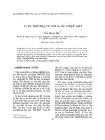
3.BEAM PROBLEM
Finite element idealisation:
Uniform load q (KN/mm)
Length unit: mm
200
200
20 4x40 20
Layered beam cross-section
1
2
3
4
5
6
Layer number
1
x
z
10
11
21 34567892345678910
10x300=3000

Uniform load q (KN/mm)
300 300 300 300 300 300 300 300 300 300
3000
Length unit: mm
200
200

20 20
Layered beam cross-section
1-2
3
Layer number
1234567891011
12345678910
x
z
8x20
10
11-12

U niform load q (K N /m m )
Length unit: m m
200
200
20 4x40 20
Layered beam cross-section
1
2
3
4
5
6
Layer number
1
x
z
20x150=3000

2
21
203 19
123 2019

Uniform load q (KN/mm)
30x100=3000
Len
g
th unit: mm
200
200
20 4x40 20
La
y
ered beam cross-section
1
2
3
4
5
6
Layer number
1
31
x
z
1
234
302928

30

Uniform load q (KN/mm)
300 300 300 300 300 300 300 300 300 300
3000
Length unit: mm
200
200
20 20
Layered beam cross-section
1
Layer number
1234567891011
12345678910
x
z
2x80
4
3
2

Fig. 1. Finite element idealisation of meshes M1, M2, M3, M4, M5
Science & Technology Development, Vol 9, No.8- 2006
Trang 8

0 5 10 15 20 25 30 35 40 45
0
0.05
0.1
0.15

0.2
0.25
0.3
0.35
0.4
0.45
Load-displacement of meshes M1, M2, M3 and refered results
b
Uniform load q (KN/mm)
Displacement U (mm)
Mesh M1
Mesh M2
Mesh M3
Owen's FE (refered from bokk [2],page 15
0

Fig. 2. Uniform load – displacement curves for meshes M
1
, M
2
, M
3
and Owen’s FE
Table 1. Distribution of plastic layers of some sections at elements with various uniform load
of mesh M2
Uniform
load (kN/mm)
0.3775
0.4280
0.4375

4321
Legend:
Elastic zone
Plastic zone
5
Element number















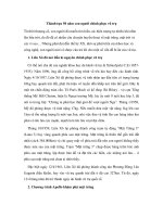
Fig. 3. Uniform load – displacement curves for meshes M2, M4 and M5
Table2. Comparison of displacement at mid-point of the beam with formulation of shear
stiffness matrix [Ks] computed with 1-Gauss point and 2-Gauss point rule of mesh M2
(tolerance
ε
D
= 10
-3
)

Uniform Displacement U (mm) Error (%)
load q 1-Gauss point 2-Gauss point
(kN/mm) (a) (b)
a-b
0.4290 10.70154906 10.63478666 0.623857
0.4320 12.31206323 12.13690619 1.422646
0 5 10 15 20 25 30 35 40
0
0.05
0.1
0.15
0.2
0.25
0.3
0.35
0.4
0.45
Displacement U (mm)
Unifo rm load q (KN/mm)
Load-displacement of meshes M2, M4, M5
Mesh M2
Mesh M4
Mesh M5

TẠP CHÍ PHÁT TRIỂN KH&CN, TẬP 9, SỐ 8 -2006
Trang 9
0.4325 12.83619912 12.57407891 2.042039
0.4365 19.45118787 18.37697980 5.522583
0.4370 20.46772651 19.30164554 5.697169

The Timoshenko beam theory has got a difficulty by using the shear stiffness matrix [Ks]
because it may lead to “locking” phenomenon with 2-point Gauss-Legendre rule formulation.
4. PLANE STRAIN AND AXISYMMETRIC PROBLEMS IN SOLID MECHANICS
APPLICATIONS
4.1. Problem description: Thick-walled cylinder under internal pressure problem

2b=400
2a=200 100100
p

Fig. 4. A thick-walled cylinder under

Material properties:
Elastic modulus: E = 2.1e4 dN/mm
2

Poissons ratio:
ν
= 0.3
Uniaxial yield stress:
σ
y = 24.0 dN/mm
2

Strain hardening parameter: H’ = 0.0
Geometry proportions:
Internal radius: a = 100 mm
External radius: b = 200 mm

01
100 5x20=100
20
z
r
13 3 14 5 15 7 16 9 17 11
2468
10
12
24 25 26 27 28
18 19 20 21 22 23
p=20 (dN/mm )
2

2
p=20 (dN/mm )
20
0
z
100
r
10x10=100

Fig. 5. Finite element idealisation of axisymmetric
problem, mesh AM1
Fig. 6. Finite element idealisation of axisymmetric
problem, mesh AM2


x

100mm
200mm
y
p

Fig. 7. Finite element idealisation of plane strain problem, mesh PM1
Science & Technology Development, Vol 9, No.8- 2006
Trang 10

0 0.05 0.1 0.15 0.2 0.25 0.3 0.35
0
2
4
6
8
10
12
14
16
18
20
Internal pressure p (dN/mm2)
Radial displacement of inner surface Ua (mm)
Mesh AM1
Mesh PM1
Owen's FE, book [2], page 262

Fig. 8. Radial displacement Ua(mm) of inner face of Mesh AM1, PM1 and Owen’s FE
100 110 120 130 140 150 160 170 180 190 2
0

4
6
8
10
12
14
16
18
Mesh AM2
Owen's FE, book [2]
Mesh PM1
Circuferential stress (dN/mm2)
Radius (mm)
p=8 dN/mm2
p=12 dN/mm2

Fig. 9. Comparison of distribution of circumferential stress
σ
θ
with internal pressure variables p=8 and
12(dN/mm
2
) of mesh AM2, PM1 and Owen’s FE.

100 110 120 130 140 150 160 170 180 190 200
8
10
12
14
16

18
20
22
24
Circumferential stress (dN/mm2)
Radius
(
mm
)

Owen's FE, book [2]
Mesh AM2
Mesh PM1
p=18 dN/mm2
p=14 dN/mm2


Fig. 10. Comparison of distribution of circumferential stress
σ
θ
with internal pressure variables p=14
and 18(dN/mm
2
) of mesh AM2, PM1 and Owen’s FE
TẠP CHÍ PHÁT TRIỂN KH&CN, TẬP 9, SỐ 8 -2006
Trang 11
5. CONCLUSION
For the Timoshenko beam problem, the analysis of elasto-plastic behaviour of the beam
considered development of plastic zone in beam sections through determining plastic layers.
However, the Timoshenko beam theory has met a difficulty by using the shear stiffness matrix

[Ks] because it may lead to “locking” phenomenon with 2-point Gauss-Legendre rule
formulation. This phenomenon can be cured by using 1-point Gauss-Legendre rule formulation
for the shear stiffness matrix. The obtained solutions are sensitive with meshes. The more
number of layers is the more stiffness of the beam. Unfortunately, the experimental results are
not available to compare with the obtained solutions by this approach.
For the considered 2-D problem, the results obtained from the present FE of several
meshes, even for coarse mesh, is close. However, the obtained results of meshes of the
axisymmetric problem model are different with the results obtained by the plane strain problem
model. The variation stress was rather smooth without concentration of stress.
The modelisation of axisymmetric problem with each element having differential stiffness
matrix is especially adaptive for analyzing some thick-walled pipes structures made by
composite material! Elements containing differential material properties have differential
stiffness or they have differential stiffness matrix.
Application of the models can be used to analyse elasto-plastic behaviour for some thick-
walled pipes made by composite materials (especially reinforced concrete pipes) and
“sandwich” materials.
PHƯƠNG PHÁP PHẦN TỬ HỮU HẠN TRONG PHÂN TÍCH GIỚI HẠN ĐÀN
HỒI - DẺO CỦA MỘT SỐ BÀI TOÁN CẤU TRÚC
Truong Tich Thien
(1)
, Cao Ba Hoang
(2)
(1) University of Technology, VNU-HCM
(2) Ministry of Construction

TÓM TẮT: Phương pháp phần tử hữu hạn được sử dụng rộng rãi trong việc phân tích
ứng xử đàn
−
dẻocủa các cấu trúc. Việc phân tích thường bao gồm quá trình hai giai đoạn: xác
định trường nội lực tác động lên vật liệu cấu trúc và đáp ứng của vật liệu ứng với trường nội

lực đó. Nói cách khác, việc phân tích các ứng xử của cấu trúc là sự thiết lập những mối quan
hệ giữa ứng suất và biến dạng trong cấu trúc biến dạng dẻo cũng như
đàn hồi. Nó đưa đến
những đánh giá thực hơn các khả năng chịu tải của các cấu trúc và cung cấp sự hiểu biết tốt
hơn về phản ứng của các phần tử kết cấu đối với những nội lực bên trong vật liệu.
REFERENCES
[1]. W. F. Chen, D. J. Han, Plasticity for Structure Engineers, Springer-Verlag- New York -
Berlin - Heidelberg - London - Paris – Tokyo, 1988.
[2]. D.R.J. Owen and E. Hinton, Finite Elements in Plasticity, Pineridge Press Limited, 54
Newton Road, Mumbles, Swansea SA3 4BQ, U.K, 1998.
[3]. L. M. Kachanov., Foundations of The Theory of Plasticity, North-Holland publishing
company - Amsterdam – London, 1971.
[4]. Prof. J. F. Debongnie, Lectures notes on Finite Element Method. University of Liège,
1999.
Science & Technology Development, Vol 9, No.8- 2006
Trang 12
[5]. M. A. Crisfield, Non-Linear Finite Element Analysis of Solid and Structure, John Wiley
& Sons, Chichester - New York - Brisbance - Toronto – Singapore, 1997.
[6]. P. G. Bergan, K. J. Bathe, W. Wunderlich, Finite Element Method for Nonlinear
Problems, Springer-Verlag- Berlin - Heidelberg - New York – Tokyo, 1996.
[7]. J. Chakrabarty, Theory of Plasticity, McGraw-Hill Book Co-Singapore, 1998.
[8]. Prof. Dr. Nguyen Dang Hung, Cours Avance De Mecanique Des Solides et Des
Structures, LTAS-Mecanique de la Rupture Universite de Liege, Belgique, 1999.
[9]. M. J. Fagan, Finite Element Analysis – Theory and Practice, Longman Singapore
Publishers (Pte) Ltd, 1992.