Báo cáo nghiên cứu khoa học " Computing vertical profile of temperature in the SOUTH-China SEA using Cubic Spline functions " docx

Pham Hoang Lam, Ha Thanh Huong, Pham Van Huan - Computing vertical profile of temperature in Eastern
Sea using cubic spline functions. Vietnam National University, Hanoi, Journal of Science, Earth Sciences,
Volume 23, No. 2, 2007, pp. 122-125


Computing vertical profile of temperature
in the SOUTH-China SEA using Cubic Spline functions


Pham Hoang Lam, Ha Thanh Huong, Pham Van Huan
University of natural sciences, VNU


Abstract: In this text the spline approximation was applied to the empirical
vertical profiles of oceanographic parameters such as temperature, salinity or
density to obtain a more precious and reliable result of interpolation. Our
experiments with the case of observed temperature profiles in the East sea show
that the cubic polynomial spline method has a higher reliability and precision in
comparison with the linear interpolation and other traditional methods. The
method was realized into a subroutine in our programs of management and
manipulation of oceanographic data.
As an application, the observed temperature field from World Ocean Data
Base 2001 consisting of about 137000 vertical profiles have been analyzed to
examine the features of the vertical distribution of temperature in the East sea.
It is found that the upper homogeneous layer in the summer months is only
a thin one with the thickness of about 10 m, but in the winter months this layer
expands to the depth of about 50-60 m and even more. And the thickness of
upper mixing layer changes largely from year to year as well with a range from
about 20 m to about 70 m.

Temperature is always an important

factor in the research of physics in
general and particular in oceanography.
With the rapid development of the
information technology, the computation
and prediction of the oceanographic
parameters are of special interest. Sea
water temperature is an important part
of the input of the modern thermo-
dynamical model. In many application,
the water temperature and other
oceanographic parameters at different
horizons are required to be calculated
from their observed profiles by the
interpolation procedures. The spline
method of approximation appears to be a
reliable and precious one for these
purposes (Belkin I. M. et all, 1982; Belkin I.
M., 1986a, 1986b; Belkin I. M., 2001).
The purpose of the cubic spline
function method is to find a cubic
polynomial on each interval on a given
coordinate line, in our case, is the z-
coordinate of depth. Suppose that on the
interval [a, b] of the z-coordinate we
have a computation grid
. At each knot, the
values of the temperature functio
n
at the layer which ha
ve been measured

[2-5] are given by
{}
. The
interpolation and extrapolation problem
using piece-wise cubic functions is to
find a function which satisfy the
following conditions (
Schoenberg I. J.,
1964
):
bzzza
n
=<<<=
10
)(zf
)(zT
n
k
T
0
k
=
- belongs to , that is
continuous together with its first and
second derivatives.
)(zf ) ,(
2
baC
- On each
interval , the

function is a cubic polynomial of
the form:
] ,[
1 kk
zz
−
)(zf
() () ( )

=
−==
3
0
)(
,
l
l
k
k
lk
zzazfzf
. (1)
nk , ,2 ,1=
- Condition
s at the knot of the grid:
kk
Tzf =)( , (2) nk , ,1 ,0=
- The second derivative
satisfies the conditions:

)(zf
′′
)()( bfaf
′′
=
′′
(3)
This problem leads to a problem of
solving a system of linear equations of
the coefficients , :
)(
2
k
a ) , ,1 ,0( nk =
)()(2
)1(
2
1
)(
2
1
)1(
2
kfahahhah
k
k
k
kk
k
k

=+++
+
++
−
,
1 , ,2 ,1 −= nk , (4)
where
0
)0(
2
=a , , (5) 0
)(
2
=
n
a






−
−
−
=
+
+−
1
11

3
k
kk
k
kk
k
h
TT
h
TT
F
,
nk , ,2 ,1= (6)
and
1−
−=
kkk
xxh . (7)
The remaining coefficients of the
system (1) are determined from the
following:
k
k
Ta =
)(
0
(8)
()
k
kk

kk
k
k
h
TT
aa
h
a
−
++−=
−
−
1
)(
2
)1(
2
)(
1
2
3
(9)
k
kk
k
h
aa
a
3
)(

2
)1(
3
)(
3
−
=
−
(10)
The solution of the problem is
assumed to be exist and unique. The
main difficulty in the setting up of the
interpolation problem using spline
function is to find the right boundary
conditions. In the interpolation problem
using data from the hydrological
stations, the boundary condition (3) is
quite suitable with the physical
environment.
To fulfill the experiments with the
spline method we use the observed
profiles of water temperature in the
South-china sea in the database World
Ocean Atlas 2001.
The temperature field is given for
the horizons 0, 10, 20, 30, 50, 75, 100,
125, 150, 200, 250, 300, 400, 500, 600,
800 and 1000 m.
Using the cubic spline functions we
have computed the temperature values

from the surface layer to the 1000 m
layer at different layer of distance 5 m
will gives us the cubic polynomials at
the intervals [ ], [ ], , [ ].
For the vertical profile of temperature at
the point of latitude 13
o
N and longitude
110
o
E, the computed coefficients of the
polynomial for each of 16 depth intervals
are listed in the table 1.
10
, zz
21
, zz
nn
zz ,
1−
From these polynom
ials one can
compute the values of the temperature
at any layer through the system of
coefficients .
310
,, aaa
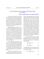
From the comparing two methods,
the traditio
nal linear interpolation and

the interpolation using cubic spline
functions, we can see the advantage of
the later one. The cubic spline functions
give smoother curve of profiles and the
profiles reflect better the variation
characteristics of temperature at
different depth (fig. 1).


Table 1: Values of the coefficients of the cubic spline function at the dividing point
at different depths
0
a
1
a
2
a
3
a
24.88 -0.000853 0.000128 -0.000004
24.89 -0.000014 -0.000212 0.000011
24.87 0.003910 -0.000181 -0.000001
24.87 -0.011432 0.000948 -0.000019
24.77 0.059762 -0.003820 0.000064
21.80 0.138229 0.000744 -0.000061
19.05 0.072143 0.001899 -0.000015
17.98 0.031601 -0.000278 0.000029
16.07 0.037510 0.000160 -0.000003
14.59 0.026389 0.000017 0.000001
13.34 0.023050 0.000050 0.000000

11.50 0.014124 0.000039 0.000000
10.24 0.011778 -0.000007 0.000000
9.05 0.011425 0.000011 0.000000
7.37 0.004491 0.000024 0.000000
6.72 0.001652 0.000000 0.000000

0
100
200
300
400
10 15 20 25
0
100
200
300
400
10 15 20 25
0
100
200
300
400
10 15 20 25
a)
b) c)
Fig. 1. Vertical distribution of temperature at point 13
o
N-110
o

E
a) measured, b) cubic spline method, c) linear interpolation


Fig. 2. Vertical distribution of
temperature (22
o
N-116
o
E

)
Fig. 3. Vertical distribution of
temperature (19
o
N-112
o
E)
Fig. 4. Vertical distribution of
temperature (16
o
N-109.5
o
E)
Fig. 5. Vertical distribution of
temperature (13
o
N

- 110

o
E)
Fig. 6. Vertical distribution of
temperature (10
o
N - 109.5
o
E)
Table 2. The seasonal changes of the homogeneous layer in 1966
at point 109
o
E - 17
o
N
Month 1 2 3 4 5 6 7 8 9 10 11 12
Thickness (m) 62 60 40 10 10 15 15
−
22 50 60 60
at point 114
o
E - 13
o
N
Month 1 2 3 4 5 6 7 8 9 10 11 12
Thickness (m) 60 65 66 45 20
−
30 30 50 40
− −
at point 109
o

E - 11
o
N
Month 1 2 3 4 5 6 7 8 9 10 11 12
Thickness (m) 25
− − −
10 8 5
−
15 30 50
−

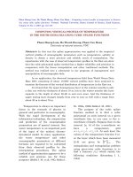
Figures 2 to 6 show the computed
profiles of some other points in the East
sea as the examples.
In general, temperature tends to
decrease as the depth increases. However
the analysis of the vertical profile of
0
50
100
150
15 20 25
0
50
100
150
15 20 25
0
50
100

150
15 20 25
0
50
100
150
15 20 25
0
50
100
150
15 20 25
temperature at these points shows the
existence of the strongly mixed layers. At
these points, the temperature is quite
homogeneous, the strong mixing even
makes the temperature at some layers
higher than the surface temperature.
These points belong to the mainly stream
area, the current speed can be as high as
1m/s at surface, so the sea water will be
mixed up strongly. The thickness of this
mixing layer is often about 50-70 m.
Under this mixing layer is the layer with
the strong variation in temperature. The
temperature begins to decrease fast until
150-200 m and after that it decreases
gradually to the bottom. This is also the
common law of changing of temperature
of sea water with depth.

Base on the analyzed vertical
profiles of temperature we can evaluate
the variability of the upper homogeneous
layer (table 2). It is clear that in the
summer months the upper homogeneous
layer is only a thin one with the
thickness of about 10 m, in the winter
months - this layer stretches to the depth
of about 50-60 m and even more.

The changes of the thickness of the
homogeneous layer between the years can
be seen by comparison the analyzed
vertical profiles at a point in winter in
some years (table 3).
Table 3. The changes of the winter homogeneous layer thickness between years
at point 112
o
E - 12
o
N
Year 1966 1969 1972 1980 1982 1989
Thickness (m) 66 38 40 50 22 65

This paper is completed with the
support of the Fundamental Research
Program, Theme Code: 705506.
References
1. Belkin I. M. et all, 1982. The space-
temporary changes of the structure of

the ocean active layer in the region of
POLYMODE Experiment. In Bulletin: 2-
nd Federal Conference of oceanographers.
Thesis of reports, Vol. 1, Pub. MGI,
Ucraina Sci. Acad., Sevastopol, p. 15-16.
(in Russian).
2. Belkin I. M., 1986a. Obective
morphologo-statistical Classification of
the vertical profiles of hydrophysical
parameters. Rep. L. 11 USSR, Part. 286,
N. 3, p. 707-711 (in Russian).
3. Belkin I. M., 1986b. Characteristic
profiles. In book: Atlas of POLYMODE.
Red. L. D. Vuris, V. M. Kamenkovich, L.
S. Monin. Woods Holl, Woods Holl
Oceanographical Ins. p. 175, 183-184 (in
Russian).
4. Belkin I. M., 2001. Morphologo-
statistical analysis of stratification of
oceans. Pub. "Hydrometeoizdat",
Leningrad, 134 p. (in Russian).
5. Schoenberg I, J., 1964. Spline function
and the problem of graduation. Pro. Nat.
USA.

Sử dụng hm spline bậc ba để tính trắc diện thẳng đứng
của nhiệt độ nớc biển Đông

Phạm Hong Lâm, H Thanh Hơng, Phạ
m Văn Huấn

Trờng Đại học Khoa học Tự nhiên, ĐHQG H Nội
Xấp xỉ spline bậc ba đợc áp dụng đối với các trắc diện thẳng đứng thực nghiệm của các
tham số hải dơng học để nhận đợc kết quả nội suy chính xác v tin cậy hơn. Thí nghiệm
của chúng tôi cho thấy rằng phơng pháp spline đa thức bậc ba có độ tin cậy v chính xác hơn
so với phơng pháp nội suy tuyến tính. Phơng pháp đã đợc hiện thực hóa thnh thủ tục
trong các chơng trình quản lý v thao tác dữ liệu hải dơng học của chúng tôi.
Với t cách ứng dụng phơng pháp, các trắc diện nhiệt độ thẳng đứng quan trắc lấy từ cơ
sở dữ liệu nhiệt độ nớc biển Đông trong World Ocean Data Base 2001 gồm 137000 trắc diện
thẳng đứng nhiệt độ đã đợc phân tích để xem xét đặc điểm phân bố nhiệt độ thẳng đứng của
vùng biển biến đổi trong năm v giữa các năm.
Thấy rằng lớp đồng nhất nhiệt độ phía trên của biển trong các tháng mùa hè chỉ l một
lớp mỏng dy khoảng 10 m, nhung trong các tháng mùa đông lớp ny mở rộng tới độ sâu 50-
60 m v thậm chí hơn. Độ dy của lớp ny cũng biến đổi mạnh từ năm ny tới năm khác với
dải biến thiên từ 20 m tới 70 m.

Địa chỉ liên hệ: Phạm Văn Huấn
334, Nguyễn Trãi, Thanh Xuân, H Nội
Điện thoại: 854945, 0912 116 661