Networking Theory and Fundamentals - Lecture 11 pot
Bạn đang xem bản rút gọn của tài liệu. Xem và tải ngay bản đầy đủ của tài liệu tại đây (326.58 KB, 37 trang )
1
TCOM 501:
Networking Theory & Fundamentals
Lecture 11
April 16, 2003
Prof. Yannis A. Korilis
2
Topics
Routing in Data Network
Graph Representation of a Network
Undirected Graphs
Spanning Trees and Minimum Weight Spanning Trees
Directed Graphs
Shortest-Path Algorithms:
Bellman-Ford
Dijkstra
Floyd-Warshall
Distributed Asynchronous Bellman-Ford Algorithm
3
Introduction to Routing
What is routing?
The creation of (state) information in the network to enable efficient delivery
of packets to their intended destination
Two main components
Information acquisition: Topology, addresses
Information usage: Computing “good” paths to all destinations
Questions
Where is B?
How to reach B?
How to best reach B?
How to best distribute all traffic
(not only A to B)?
A
E
C
D
F
B
G
4
Graph-Theoretic Concepts
An Undirected Graph G = (N, A) consists of:
a finite nonempty set of nodes N and
a collection of “arcs” A, interconnecting pairs
of distinct nodes from N.
If i and j are nodes in N and (i, j) is an arc in
A, the arc is said to be incident on i and j
Walk: sequence of nodes (n
1
, n
2
, …, n
k
),
where (n
1
, n
2
), (n
2
, n
3
), …, (n
k-1
, n
k
) are arcs
Path: a walk with no repeated nodes
Cycle: a walk (n
1
, n
2
, …, n
k
), with n
1
=n
k
and
no other repeated nodes
Connected Graph: for all i, j∈ N, there exists
a path (n
1
, n
2
, …, n
k
), with i=n
1
, j=n
k
A
E
C
D
F
B
G
{, , , , , , }
{( , ),( , ),( , ),( , ),
( , ),( , ),( , )}
A
BCDEFG
A
EACCDCF
BD BG EG
=
=
N
A
5
Spanning Tree
A graph G' = (N ', A' ), with N '⊆ N and A'⊆ A is called a subgraph of G
Tree: a connected graph that contains no cycles
Spanning tree of a graph G: a subgraph of G, that is a tree and contains all
nodes of G, that is N ' = N
Lemma: Let G be a connected graph G = (N, A) and S a nonempty strict
subset of the set of nodes N. Then, there exists at least one arc (i, j) such
that i∈S, and j∉S.
A
E
C
D
F
B
G
6
Spanning Tree Algorithm
1. Select arbitrary node n∈N, and initialize: G' = (N ', A' ),
2. If N' = N, STOP: G' = (N ', A' ) is a spanning tree
ELSE: go to step 3
3. Let (i, j) ∈ A with i ∈ N' and j ∈ N-N'
Update:
Go to step 2
Proof of correctness: Use induction to establish that after a new node i
is added, G' remains connected and does not contain any cycles –
therefore, it is a tree. After N-1 iterations, the algorithm terminates, and
G' contains N nodes and N-1 arcs.
{},n
′
′
=
=∅NA
:{},:{(,)}jij
′′ ′′
=∪ =∪NN AA
7
Construction of a Spanning Tree
N'= {A}; A'= ∅
N'= {A,E}; A'= {(A,E)}
N'= {A,E,C};
A'= {(A,E),(A,C)}
N'= {A,E,C,D};
A'= {(A,E),(A,C),(CD)}
N'= {A,E,C,D,F};
A'= {(A,E),(A,C),(CD),(CF)}
N'= {A,E,C,D,F,B};
A'= {(A,E),(A,C),(CD),(CF),(F,B)}
N'= {A,E,C,D,F,B,G};
A'= {(A,E),(A,C),(CD),(CF),(F,B),(E,G)}
A
E
C
D
F
B
G
8
Spanning Trees
Proposition: Let G be a connected graph with N nodes and A links
1. G contains a spanning tree
2. A ≥ N-1
3. G is a tree if and only if A=N-1
Proof: The spanning tree construction algorithm starts with a single
node and at each iteration augments the tree by one node and one arc.
Therefore, the tree is constructed after N-1 iterations and has N-1 links.
Evidently A ≥ N-1.
If A=N-1, the spanning tree includes all arcs of G, thus G is a tree.
If A>N-1, there is a link (i, j) that does not belong to the tree. Considering
the path connecting nodes i and j along the spanning tree, that path and
link (i, j) form a cycle, thus G is not a tree.
9
Use of Spanning Trees
Problem: how to distribute information to all nodes in a graph (network) –
e.g., address and topology information
Flooding: each node forwards information to all its neighbors. Simple, but
multiple copies of the same packet traverse each link and are received by
each node
Spanning tree: nodes forward information only along links that belong to the
spanning tree. More efficient:
Information reaches each node only once and traverses links at most once
Note that spanning tree is bidirectional
A
E
C
D
F
B
G
10
Minimum Weight Spanning Tree
5
2
3
1
6
7
2
3
4
21W
=
A
E
C
D
F
B
G
Weight w
ij
is used to quantify the “cost” for
using link (i, j)
Examples: delay, offered load, distance, etc.
Weight (cost) of a tree is the sum of the
weights of all its links – packets traverse all
tree links once
Definition: A Minimum Weight Spanning Tree
(MST) is a spanning tree with minimum sum
of link weights
Definition: A subtree of an MST is called a
fragment. An arc with one node in a fragment
and the other node not in this fragment is
called an outgoing arc from the fragment.
A
E
C
D
F
B
G
5
2
3
1
6
7
2
3
4
15W
=
11
Minimum Weight Spanning Trees
Lemma: Given a fragment F, let e=(i, j) be an
outgoing arc with minimum weight, where j∉F.
Then F extended by arc e and node j is a fragment.
Proof:
Let T be the MST that includes fragment F. If e∈T,
we are done.
Assume e∉T: then a cycle is formed by e and the
arcs of T
Since j∉F. there is an arc e’≠e which belongs to the
cycle and T, and is outgoing from F.
Let T’=(T-{e’}) ∪{e}. This is subgraph with N-1 arcs
and no cycles (since j∉F), i.e., a spanning tree.
Since w
e
≤w
e’
, the weight of T’ is less than or equal to
the weight of T
Then T’ is an MST, and F extended by arc e and node
j is a fragment.
A
E
C
D
F
B
G
4
4
3
1
6
7
2
3
4
e
'e
F
12
Minimum Weight Spanning Tree Algorithms
Inductive algorithms based on the previous lemma
Prim’s Algorithm:
Start with an arbitrary node as the initial fragmant
Enlarge current fragment by successively adding minimum weight outgoing
arcs
Kruskal’s Algorithm:
All vertices are initial fragments
Successively combine fragments using minimum weight arcs that do not
introduce a cycle
13
Prim’s Algorithm
C
D
E
F
A
B
1
2
3
9
75
6
8
4
C
D
E
F
A
B
C
D
E
F
A
B
C
D
E
F
A
B
C
D
E
F
A
B
C
D
E
F
A
B
C
D
E
F
A
B
14
Kruskall’s Algorithm
C
D
E
F
A
B
1
2
3
9
75
6
8
4
C
D
E
F
A
B
C
D
E
F
A
B
C
D
E
F
A
B
C
D
E
F
A
B
C
D
E
F
A
B
C
D
E
F
A
B
15
Shortest Path Algorithms
Problem: Given nodes A and B, find the “best” route for sending
traffic from A to B
“Best:” the one with minimum cost – where typically the cost of a
path is equal to the sum of the costs of the links in the path
Important problem in various networking applications
Routing of traffic over network links ⇒ need to distinguish direction
of flow
Appropriate network model: Directed Graph
16
Directed Graphs
A Directed Graph – or Digraph – G = (N, A) consists of:
a finite nonempty set of nodes N and
a collection of “directed arcs” A, i.e., ordered pairs of distinct nodes from N.
Directed walks, directed paths and directed cycles can be defined to
extend the corresponding definitions for undirected graphs
Given a digraph G = (N, A), there is an associated undirected graph G' =
(N ', A' ), with N '=N and (i, j)∈A' if (i, j)∈A, or (j, i)∈A
A digraph G = (N, A) is called connected if its associated undirected
graph G' = (N ', A' ) is connected
A digraph G = (N, A) is called strongly connected if for every i, j∈ N,
there exists a directed path (n
1
, n
2
, …, n
k
), with i=n
1
, j=n
k
17
Shortest Path Algorithms – Problem Formulation
Consider an N vertex graph G = (N, A) with link lengths d
ij
for edge (i,j) (d
ij
= ∞ if (i,j) ∉ A)
Problem: Find minimum distance paths from all vertices in
N to vertex 1
Alternatively, find minimum weight paths from vertex 1 to all vertices
in N
General approach is again iterative
Differences are in how the iterations proceed
Three main algorithms
}min{
)()1(
ij
n
j
n
i
dDD +=
+
18
Bellman-Ford Algorithm
Iterative step is over increasing hop count
Define D
i
h
as a shortest walk from node i to 1
that contains at most h edges
D
1
h
= 0 by definition for all h
Bellman-Ford Algorithm
Define
Set initial conditions to D
i
0
= ∞ for i ≠ 1
a The scalars D
i
h
are equal to the shortest walk lengths
with less than h hops from node i to node 1
b The algorithm terminates after at most N iterations if
there are no negative length cycles without node 1,
and it yields the shortest path lengths to node 1
1 },{min
1
≠∀+=
+
idDD
ij
h
j
j
h
i
19
Proof of Bellman-Ford (1)
Proof is by induction on hop count h
For h = 1 we have
D
i
1
= d
i1
for all i ≠ 1, so the result holds for i = 1
Assume that the result holds for all k ≤ h. We need to
show it still holds for h+1
Two cases need to be considered
1 The shortest (≤ h+1) walk from i to 1 has ≤ h edges
Its length is then D
i
h
2 The shortest (≤ h+1) walk from i to 1 has (h+1) edges
It consists of the concatenation of an edge (i,j) followed by a
shortest h hop walk from vertex j to vertex 1
This second case is the one we will focus on
20
Proof of Bellman-Ford (2)
From Case 1 and Case 2, we have
From induction hypothesis and initial conditions
D
i
k
≤ D
i
k-1
for all k ≤ h so that
D
i
h
≤ D
i
1
= d
i1
= d
i1
+ D
1
h
Combining the two gives
which completes the proof of part a
[]
{
}
ij
h
j
j
h
i
dDDh +=+≤
≠1
min,minlength walk )1(shortest
[]
{
}
{}
11
,min
min,minlength walk )1(shortest
++
==
+=+≤
h
i
h
i
h
i
ij
h
j
j
h
i
DDD
dDDh
[
]
[
]
h
iij
h
j
j
ij
h
j
j
h
i
DdDdDD =+≤+=
−+ 11
minmin
21
Proof of Bellman-Ford (3)
Assume that the algorithm terminates after h steps
This implies that D
i
k
= D
i
h
for all i and k ≥ h
This means that adding more edges cannot decrease
the length of any of those walks
Hence, there cannot be negative length cycles that do
not include node 1
They could be repeated many times to make walk lengths
arbitrarily small
Delete all such cycles
This yields paths of less than or equal length
So for all i we have a path of h hops or less to vertex 1 and
with length D
i
h
Since those paths have no cycles they contain at most N-1
edges,and therefore D
i
N
= D
i
N-1
for all i
The algorithm terminates after at most N steps,
which proves part b
22
Bellman-Ford Complexity
Worst-case amount of computation to find
shortest path lengths
Algorithm iterates up to N times
Each iteration is done for N-1 nodes (all i ≠ 1)
Minimization step requires considering up to N-1
alternatives
⇒ Computational complexity is O(N
3
)
More careful accounting yields a computational
complexity of O(hM)
23
Constructing Shortest Paths
B-F algorithm yields shortest path lengths,
but we are also interested in actual paths
Start with B-F equation
For all vertices i ≠ 1 pick the edge (i,j) that
minimizes B-F equation
This generates a subgraph with N-1 edges (a tree)
For any vertex i follow the edges from vertex i
along this subgraph until vertex 1 is reached
Note: In graphs without zero or negative
length cycles, B-F equation defines a system
of N-1 equations with a unique solution
[]
0 and ,1 ,min
1
=≠∀+=
∈
DidDD
ijj
Gj
i
24
Constructing Shortest Paths
D
A
= 3 + D
E
D
E
= 4 + D
G
D
G
= 3 + D
B
= 3
D
D
= 2 + D
G
D
C
= 1 + D
D
D
F
= 6 + D
B
= 6
AB = A-E-G-B
B
A
C
D
E
F
G
3
4
2
7
3
6
4
1
4
25
Dijkstra’s Algorithm (1)
Different iteration criteria
Algorithm proceeds by increasing path length instead
of increasing hop count
Start with “closest” vertex to destination, use it to find the
next closest vertex, and so on
Successful iteration requires non-negative edge
weights
Dijkstra’s algorithm maintains two sets of vertices
L: Labeled vertices (shortest path is known)
C: Candidate vertices (shortest path not yet known)
One vertex is moved from C to L in each iteration