Networking Theory and Fundamentals - Lecture 8 potx
Bạn đang xem bản rút gọn của tài liệu. Xem và tải ngay bản đầy đủ của tài liệu tại đây (284.32 KB, 24 trang )
1
TCOM 501:
Networking Theory & Fundamentals
Lecture 8
March 19, 2003
Prof. Yannis A. Korilis
8-2
Topics
Closed Jackson Networks
Convolution Algorithm
Calculating the Throughput in a Closed Network
Arrival Theorem for Closed Networks
Mean-Value Analysis
Norton’s Equivalent
8-3
Closed Jackson Networks
1
µ
2
λ
3
µ
4
µ
5
µ
1
λ
2
µ
4
λ
3
λ
5
λ
51
r
53
r
M
Closed Network: K nodes with exponential servers
No external arrivals (γ
i
=0) , no departures (r
i0
=0)
Fixed number M of circulating customers
Appropriate model for systems with “limited” resources, e.g., flow
control mechanisms
Steady-state distribution will be shown to be of “product-form” type
8-4
Closed Jackson Network
Aggregate arrival rates
Relative arrival rates – visit ratios
Can only be determined up to a constant
Use an additional equation to obtain unique solution to the above system, e.g.
Set λ
j
=1, for some node j
Set λ
j
=µ
j
, for some node j
Set λ
1
+ λ
2
+…+ λ
K
=1
n
i
: number of customers at node i
Possible states for the closed network n=(n
1
, n
2
,…,n
K
), with
Let F(M) denote the set of all such states
1
µ
2
λ
3
µ
4
µ
5
µ
1
λ
2
µ
4
λ
3
λ
5
λ
51
r
53
r
M
1
,1, ,
K
ijji
j
ri K
=
λ= λ =
∑
1
0 and | |
K
ii
i
nnnM
=
≥≡=
∑
8-5
Closed Jackson Network
Let x
i
be the number of customers at station i, at steady state
Random variables x
1
, x
2
,…, x
K
are not independent – their sum must be
equal to M
The state x=(x
1
, x
2
,…, x
K
) of the closed network can take values
n=(n
1
, n
2
,…,n
K
), with
Let F(M) denote the set of all such states
Define ρ
i
≡λ
i
/µ
i
–this is not the actual utilization factor of station i
Jackson’s theorem for closed networks gives the stationary distribution
1
0 and | |
K
ii
i
nnnM
=
≥≡=
∑
11
() { } { , , }
K
K
pn Px n Px n x n
=
== = =…
8-6
Jackson’s Theorem for Closed Networks
Theorem 1: The stationary distribution of a closed Jackson network is
where the normalization constant G(M) is a function of M
G(M) guarantees that {p(n)} is a valid probability distribution
This stationary distribution is said to have a product-form
However: at steady-state the queues are not independent
{p
i
(n
i
)}: marginal stationary distribution of queue i
1
1
() , for all ( ) {: 0,| | }
()
i
K
n
ii
i
pn n M n n n M
GM
=
=ρ ∈=≥=
∏
F
() () 1
() 1 ( )
i
K
n
i
nM nMi
pn GM
∈∈=
=
⇒= ρ
∑∑∏
FF
11
() ( ) ( )
K
K
pn p n p n
≠
8-7
Jackson’s Theorem for Closed Networks (proof)
Theorem 2: The reversed chain of a stationary closed Jackson network
is also a stationary closed Jackson network with the same service rates
and routing probabilities:
Proof of Theorems 1 & 2:
Show that for the corresponding forward and reversed chains
Need to prove only for m=T
ij
n
Verify, exactly as in the open-network case, that:
*
/
ij j ji i
rr
=
λλ
*
() (,) ()(,), , ( ),
p
mq mn pnqnm nm M n m=∈≠F
** *
(,) ( ,) { 10} ( /)
ij i j j ji i j i ij j
qTnn qn e en r n r=−+ =µ +>=µλλ1
*
1
()(,) ()(,) ()( /) ()1
{
0
}
() ()1{ 0}
ij ij ij ij j i ij j i ij i
ij j i i
pTnq Tnn pnqnTn pTn r pn r n
pTn pn n
−
=
⇔µλλ=µ>
⇔=ρρ >
(, ) { 0}
ij i ij i
qnTn r n=µ >1
*
(, ) (, ) 1{ 0}, ( )
ii
mn mn i
qnm q nm n n M
≠≠
==µ>∈
∑∑ ∑
F
8-8
Closed Jackson Network
Example: Closed network model for CPU (rate µ
1
) and
I/O (rate µ
2
) system. Upon service completion in 1,
customer routed to 2 with probability p
2
=1-p
1
, or back
to 1 with probability p
1
. M =fixed number of customers
Stationary distribution: n customers in 2 and M-n in 1
Normalization constant
Utilization factor and throughput of node 1:
2
µ
2
λ
11122 21 11 2 21
, . Choose solution: and pp pλ= λ+λ λ= λ λ=µ λ= µ
21
12
2
1,
p
µ
ρ= ρ=
µ
12 2
11
( , ) , 0,1, ,
() ()
Mn n n
pM nn n M
GM GM
−
−= ρρ= ρ =
1
2
2
0
2
1
()
1
M
M
n
n
GM
+
=
−ρ
=ρ=
−
ρ
∑
2
(1)
()1 (0,)1
() ()
M
GM
UM p M
GM GM
ρ
−
=− =− =
111
(1)
() ()
()
GM
MUM
GM
−
γ= µ=µ
1
µ
1
p
1
λ
2
p
8-9
Closed Networks: Normalization Constant
Normalization constant as a function of M and K:
All performance measures of interest – throughput, average delay – can
be obtained in terms of G(M,K)
Computational complexity is exponential in M and K:
Recursive methods can be used to reduce complexity
Iterative algorithm [due to Buzen]
Normalization constant will be treated as a function of both M and K
and denoted G(M,K) only in the context of the iterative algorithm
12
1
12
() 1
0
(,)
i
K
K
i
K
n
nn n
iK
nMi n nM
n
GMK
∈= ++=
≥
=
ρ= ρρ ρ
∑∏ ∑
F
1
terms in the summation
MK
M
+
−
8-10
Iterative Computation of G(M)
For any m and k (m=0,…, M; k=1,…, K) define:
For a closed network of single-server queues G(M,K) can be computed
iteratively using the following recursive relation:
with boundary conditions:
12
1
12
() 1
(,)
ik
k
k
nn
nn
ik
nmi n nm
Gmk
∈= ++=
=
ρ= ρρ ρ
∑∏ ∑
F
(,) (, 1) ( 1,)
k
Gmk Gmk Gm k
=
−+ρ −
1
( ,1) , 0,1, ,
(0, ) 1, 1,2, ,
m
Gm m M
Gk k K
=ρ =
==
8-11
Iterative Algorithm (proof)
For
0 and 1mk>>
we split the sum into two sums over disjoint sets of states,
corresponding to
0,
k
n
=
and
0
k
n >
.
12
1
12 12
11
1
12 12
11 1
12
12 12
00
12 1 12
0
(,)
k
k
kk
kk
kk
kk
kk
k
nnn
k
nnM
nnnn nn
kk
nnm nnm
nn
nnnn nn
kk
nnm nnm
n
Gmk
−
−
++ =
++ = ++ =
=>
−
++ = ++ =
>
=ρρρ
= ρρρ+ ρρρ
=
ρρ ρ + ρρ ρ
∑
∑∑
∑∑
N
ote that the first sum is
(, 1).Gmk
−
For the second sum, observing that
0,
k
n >
we define
1,
kk
nn
′
=+
where
0.
k
n
′
≥
Then:
12 12
11
12
1
1
12 12
1
00
12
1
0
(1,)
kk
kk
kk
k
k
k
nn
nn nn
kk
nnm nnm
nn
n
nn
kkk
nnm
n
Gm k
′
+
′
++ = ++ +=
′
>≥
′
′
++ =−
′
≥
ρρ ρ = ρρ ρ
=ρ ρ ρ ρ =ρ −
∑
∑
∑
Therefore:
(,) (, 1) ( 1,)
k
Gmk Gmk Gm k
=
−+ρ −
8-12
Iterative Algorithm – Example
µ
µ
λ
4
λ
3
λ
5
λ
51
1
2
r
=
53
1
2
r
=
M
2
µ
2
µ
2
λ
1
λ
Visit ratios λ
i
determined up to a multiplicative constant
Letting λ
1
= 2µ, we have:
Calculation of G(M,5) based on the iterative algorithm using these values
1234
51 53 1 3
513 1
,
2
rr
λ=λ λ=λ
=⇒λ=λ
λ=λ+λ=λ
121 34 3 1
55 1 1
/2 , / 2
/2/4/, with /
ρ=ρ=λ µρ=ρ=λ µ=ρ
ρ=λ λ=λ λ=ρ ρ ρ≡λµ
12 34 5
1, 2, 4 /
ρ
=ρ = ρ =ρ = ρ = ρ
8-13
Iterative Algorithm – Example
Boundary conditions:
Iteration:
1 2 3 4 5
0
1 1 1 1 1
1
1 2 4 6 6+4/ρ
2
1 3 11 23 23+(6+4/ρ)(4/ρ)
3
1 4 26 72 72+[23+(6+4/ρ)(4/ρ)](4/ρ)
k
m
12 34 5
1, 2, 4 /ρ=ρ= ρ=ρ= ρ= ρ
1
( ,1) , 0,1, ,
(0, ) 1, 1,2, ,
m
Gm m M
Gk k K
=ρ =
==
(,) (, 1) ( 1,)
k
Gmk Gmk Gm k=−+ρ−
Example:
2
3
2
(1, 2) (1,1) (0, 2) 1 1 2
(1,3) (1,2) (0,3) 2 2 4
(2,2) (2,1) (1,2) 1 2 3
GG G
GG G
GG G
=
+ρ = + =
=
+ρ =+=
=
+ρ = + =
8-14
Marginal Distribution
Proposition 1: In a closed Jackson network with M customers, the
probability that at steady-state, the number of customers in station j
greater than or equal to m is:
Proof 1:
Px
()
{} ,0
()
m
jj
GM m
P
xm mM
GM
−
≥=ρ ≤≤
1
1
1
1
1
1
1
()
1
1
0
{} ()
()
()
()
()
()
j
K
jK
j
j
j
K
jK
j
j
K
jK
j
n
nn
jK
j
nM n n nM
nm
nm
nm
nn
jK
nnmnM
nmm
m
n
j
nn
jK
nn nMm
n
m
j
m pn
GM
GM
GM
GM m
GM
∈++++=
≥
≥
′
+
′
+++++ =
′
+≥
′
′
++++ = −
′
≥
ρ
ρρ
≥= =
ρρ ρ
=
ρ
=ρρρ
ρ
=−
∑∑
∑
∑
……
……
……
F
8-15
Marginal Distribution
Proposition 2: In a closed Jackson network with M customers, the
probability that in steady state there are m customers at station j is:
Proof 2:
Proposition 3: In a closed Jackson network with M customers, the average
number of customers at queue j is:
Proof 3:
P
NE
()( 1)
{} ,0
()
m
i
jj
GM m GM m
P
xm mM
GM
−
−ρ − −
==ρ ≤≤
{}{}{ 1}
jjj
xmPxmPxm== ≥− ≥+
11
()
[] { }
()
MM
m
jj j j
mm
GM m
x Pxm
GM
==
−
== ≥=ρ
∑∑
1
()
()
()
M
m
jj
m
GM m
NM
GM
=
−
=ρ
∑
8-16
Average Throughput
Proposition 4: In a closed Jackson network with M customers, the
average throughput of queue j is:
Proof 4: Average throughput is the average rate at which customers are
serviced in the queue. For a single-server queue the service rate is µ
j
when there are one or more customers in the queue, and 0 when the
queue is empty. Thus:
(1)
()
()
jj
GM
M
GM
−
γ=λ
(1) (1)
() { 1}
() ()
jjjjj j
GM GM
MPx
GM GM
−−
γ=µ≥=µ⋅ρ =λ
8-17
Example: ./M/1 Queues in Tandem
M
K
21
µ
µ
µ
()
M
γ
12 K
λ=λ= =λ…
Choose
12
1, 1, ,
Ki
iKλ=λ= =λ =µ ⇒ ρ= =…
12
12
() ()
1
(1)!
() 1
!( 1)!
K
nn n
K
nM nM
MK
MK
GM
M
MK
∈∈
+−
+
−
=ρρρ= = =
−
∑∑
FF
1
11!(1)!
( ) , for all ( )
1
() ( 1)!
i
K
n
i
i
MK
pn n M
MK
GM M K
M
=
−
=ρ= = ∈
+−
+−
∏
F
8-18
Example: ./M/1 Queues in Tandem (cont.)
Average throughput:
For queue j=1,…,K:
Average time-delay:
M
K
21
µ
µ
µ
()
M
γ
(1) ( 2)! !(1)!
() ()
( ) ( 1)!( 1)! ( 1)!
1
jj
GM M K M K
MM
GM M K M K
M
M
K
−
+− −
γ=γ =λ =µ ⋅
−
−+−
=µ
+−
()
()
11 11
()
()
j
j
j
j
M
NM
K
NM
MM K M K
TM
MK M K
=
+− +−
==⋅ =
γµµ
1
() ()
j
j
MK
TM T M
+
−
==
∑
µ
8-19
Arrival Theorem for Closed Networks
Theorem: In a closed Jackson network with M customers, the
occupancy distribution seen by a customer upon arrival at queue j is the
same as the occupancy distribution in a closed network with the arriving
customer removed.
Corollary: In a closed network with M customers, the expected number
of customers found upon arrival by a customer at queue j is equal to the
average number of customers at queue j, when the total number of
customers in the closed network is M-1.
Intuition: an arriving customer sees the system at a state that does not
include itself.
8-20
Arrival Theorem (proof)
1
( ) ( ( ), , ( ))
K
xt x t x t=
state of the network at time t
()
ij
Tt
probability that a customer moves from station i to j, at time t
+
For any state
()nM∈F
with
0
i
n >
,
find the conditional probability that a customer
moving from node i to node j finds the network at state n
1
1
()
0
1
1
() ()
00
{ () , ()} { () } { ()| () }
() {() | ()}
{
()
}{
()
}{
()
|
()
}
()
()
i
iK
iK
ii
ij ij
ij ij
ij ij
mM
m
n
nn
iij
iK
mmm
iij i K
mM mM
mm
PxtnTt PxtnPTtxtn
nPxtnTt
PT t Pxt mPT t xt m
pn r
pm r
∈
>
∈∈
>>
=
==
α= = = =
==
µ
ρρρ
==
µρρρ
∑
∑∑
F
FF
Changing index
1, 0
ii i
mm m
′
′
=
+≥
in the sum in the denominator:
1
1
1
11
1
1
1
1
1
1
10
11
11
1
1
0
()
(1)
i
K
iK
iK
i
ii
KK
iK
iK
i
n
nn
iK
ij
mmm
iK
mm mM
m
nn
nn nn
iK iK
mmm
iK
mmmM
m
n
GM
′
+
′
++ +++ =
′
+>
−−
′
′
++ ++ = −
′
≥
ρρρ
α=
ρρ ρ
ρ
ρρ ρρρ
==
ρρρ −
∑
∑
……
……
This is the probability of state
1
(, , 1, )
iK
nn n
−
……
in
an identical network with M-1
customers
8-21
Mean-Value Analysis
Closed network with M customers; performance measures
N
j
(M): average number of customers in queue j
T
j
(M): average a customer spends (per visit) in queue j
γ
j
(M): average throughput of queue j
Mean-Value Analysis: Calculates N
j
(M) and T
j
(M) directly, without first
computing G(M) or deriving the stationary distribution of the network
Iterative calculation:
with initial condition:
Average throughput
1
1(1)
( ) , 1, , ; 1, ,
()
( ) , 1, , ; 1, ,
()
j
j
j
jj
j
K
ii
i
Nm
Tm j Km M
Tm
Nm m j Km M
Tm
=
+
−
===
µ
λ
===
λ
∑
(0) 0, 1, ,
j
NjK
=
=
()
( ) , 1, , ; 1, ,
()
j
j
j
Nm
mjKmM
Tm
γ= = =
8-22
Mean Value Analysis (proof)
Arrival Theorem → expected number of customers that an arrival finds
at queue j is N
j
(m-1). Service rate for all customer at the queue µ
j
.
λ
1
,…,λ
K
: visit ratios – a solution to flow conservation equations
Actual throughput of queue j:
Using Little’s Theorem:
Summing for all j and noting that ∑
j
N
j
(m)= m:
Then:
1(1)
( ) , 1, , ; 1, ,
j
j
j
Nm
Tm j Km M
+
−
===
µ
() ( 1)/() ()
jj j
mGmGm mγ=λ − =λα
() () () () ()
jjj jj
Nm mTm m Tm
=
γ=αλ
11
1
() () () ()
()
KK
iii
K
ii
ii
i
m
mNm mTm m
Tm
==
=
==αλ⇒α=
λ
∑∑
∑
1
()
( ) , 1, , ; 1, ,
()
jj
j
K
ii
i
Tm
Nm m j Km M
Tm
=
λ
===
λ
∑
8-23
Example: ./M/1 Queues in Tandem
M
K
21
µ
µ
µ
()
M
γ
12
1, 1, ,
Ki
iKλ=λ= =λ =µ ⇒ ρ= =…
1
1(0) (1) (1)
11
(1) , (1) 1 , (1)
(1)
(1)
jjj
jj j
K
j
i
i
NTN
TN K
KT
T
=
+µ
== = =γ==µ
µµ
µ
∑
1(1) (2)
11/ 11 2 2
(2) , (2) , (2)
(2) 1
j j
jjj
j
NN
KK
TN
KKTK
+
++
=== =γ==µ
µµ µ +
1(2) (3)
12/ 21 3 3
(3) , (3) , (3)
(3) 2
j j
jjj
j
NN
KK
TN
KKTK
+
++
=== =γ==µ
µµ µ +
1(3) (4)
13/ 31 4 4
(4) , (4) , (4)
(4) 3
j j
jjj
j
NN
KK
TN
KKTK
+
++
=== =γ==µ
µµ µ +
11
() , () , ()
1
jjj
MK M M
TM NM M
KKMK
+
−
==γ=µ
µ
+−
8-24
State-Dependent Service Rates
Theorem: The stationary distribution of a closed Jackson network where
the nodes have state-dependent service rates is
where the normalization constant G(M) is a function of M, the fixed
number of customers in the network
Normalization constant:
Proof similar to the one for open networks
1
1
() , for all ( ) {: 0,| | }
() (1) ()
i
n
K
i
i
i
iii
p
nnKnnnK
GM n
=
=∈=≥=
∏
λ
µµ
F
() 1 ()
() ()1
(1) ( )
i
n
K
i
nKi nK
iii
GM pn
n
∈= ∈
λ
=
⇒=
µµ
∑∏ ∑
FF