Biosignal and Biomedical Image Processing MATLAB-Based Applications Muya phần 9 pot

Filters, Transformations, and Registration 311
dimension of the output is the sum of the two matrix lengths along that dimen-
sion minus one. Hence, if the two matrices have sizes
I1(M1, N1)
and
h(M2,
N2)
, the output size is:
I2(M1 ؉ M2 − 1, N2 ؉ N2 − 1)
. If shape is
‘valid’
,
then any pixel evaluation that requires image padding is ignored and the size of
the output image is:
Ic(M1- M2 ؉ 1, N1- N2 ؉ 1)
. Finally, if
shape
is
‘same’
the size of the output matrix is the same size as
I1
; that is:
I2(M1, N1)
. These
options allow a great deal in flexibility and can simplify the use of two-dimen-
sional convolution; for example, the
‘same’
option can eliminate the need for
dealing with the additional points generated by convolution.
Two-dimensional correlation is implemented with the routine
‘imfilter’

that provides even greater flexibility and convenience in dealing with size and
boundary effects. The calling structure of this routine is given in the next page.
I2 = imfilter(I1, h, options);
where again
I1
and
h
are the input matrices and
options
can include up to
three separate control options. One option controls the size of the output array
using the same terms as in
‘conv2’
above:
‘same’
and
‘full’
(
‘valid’
is
not valid in this routine!). With
‘imfilter’
the default output size is
‘same’
(not
‘full’
), since this is the more likely option in image analysis. The second
possible option controls how the edges are treated. If a constant is given, then
the edges are padded with the value of that constant. The default is to use a
constant of zero (i.e., standard zero padding). The boundary option

‘symmet-
ric’
uses a mirror reflection of the end points as shown in Figure 2.10. Simi-
larly the option
‘circular’
uses periodic extension also shown in Figure 2.10.
The last boundary control option is
‘replicate’
, which pads using the nearest
edge pixel. When the image is large, the influence of the various border control
options is subtle, as shown in Example 11.4. A final option specifies the use of
convolution instead of correlation. If this option is activated by including the
argument
conv
,
imfilter
is redundant with
‘conv2’
except for the options
and defaults. The
imfilter
routine will accept all of the data format and types
defined in the previous chapter and produces an output in the same format;
however, filtering is not usually appropriate for indexed images. In the case of
RGB images,
imfilter
operates on all three image planes.
Filter Design
The MATLAB Image Processing Toolbox provides considerable support for
generating the filter coefficients.* A number of filters can be generated using

MATLAB’s
fspecial
routine:
*Since MATLAB’s preferred implementation of image filters is through correlation, not convolu-
tion, MATLAB’s filter design routines generate correlation kernels. We use the term “filter coeffi-
cient” for either kernel format.
TLFeBOOK
312 Chapter 11
h = fspecial(type, parameters);
where
type
specifies a specific filter and the optional parameters are related to
the filter selected. Filter type options include:
‘gaussian’
,
‘disk’
,
‘sobel’
,
‘prewitt’
,
‘laplacian’
,
‘log’
,
‘average’
, and
‘unsharp’
. The
‘gauss-

ian’
option produces a Gaussian lowpass filter. The equation for a Gaussian
filter is similar to the equation for the gaussian distribution:
h(m,n) = e
−(d/σ)/2
where d =
√
(m
2
+ n
2
)
This filter has particularly desirable properties when applied to an image:
it provides an optimal compromise between smoothness and filter sharpness.
The MATLAB routine for this filter accepts two parameters: the first specifies
the filter size (the default is 3) and the second the value of sigma. The value of
sigma will influence the cutoff frequency while the size of the filter determines
the number of pixels over which the filter operates. In general, the size should
be 3–5 times the value of sigma.
Both the
‘sobel’
and
‘prewitt’
options producea3by3filter that
enhances horizontal edges (or vertical if transposed). The
‘unsharp’
filter pro-
duces a contrast enhancement filter. This filter is also termed unsharp masking
because it actually suppresses low spatial frequencies where the low frequencies
are presumed to be the unsharp frequencies. In fact, it is a special highpass

filter. This filter has a parameter that specifies the shape of the highpass charac-
teristic. The
‘average’
filter simply produces a constant set of weights each of
which equals 1/N, where N = the number of elements in the filter (the default
size of this filter is 3 by 3, in which case the weights are all 1/9 = 0.1111). The
filter coefficients for a 3 by 3 Gaussian lowpass filter (sigma = 0.5) and the
unsharpe filter (alpha = 0.2) are shown below:
h
unsharp
=
ͫ
−0.1667 −0.6667 −0.1667
−0.6667 4.3333 −0.6667
−0.1667 −0.6667 −0.1667
ͬ
;
h
gaussian
=
ͫ
0.0113 0.0838 0.0113
0.0838 0.6193 0.0838
0.0113 0.0838 0.0113
ͬ
The Laplacian filter is used to take the second derivative of an image:
∂
2
/∂x. The log filter is actually the log of Gaussian filter and is used to take the
first derivative, ∂ /∂x, of an image.

MATLAB also provides a routine to transform one-dimensional FIR fil-
ters, such as those described in Chapter 4, into two -dimensional filters. This
approach is termed the frequency transform method and preserves most of the
characteristics of the one-dimensional filter including the transition band-
width and ripple features. The frequency transformation method is implemented
using:
h = ftrans2(b);
TLFeBOOK
Filters, Transformations, and Registration 313
where
h
are the output filter coefficients (given in correlation kernel format),
and
b
are the filter coefficients of a one-dimensional filter. The latter could be
produced by any of the FIR routines described in Chapter 4 (i.e.,
fir1, fir2,
or
remez
). The function
ftrans2
can take an optional second argument that
specifies the transformation matrix, the matrix that converts the one-dimensional
coefficients to two dimensions. The default transformation is the McClellan
transformation that produces a nearly circular pattern of filter coefficients. This
approach brings a great deal of power and flexibility to image filter design since
it couples all of the FIR filter design approaches described in Chapter 4 to image
filtering.
The two-dimensional Fourier transform described above can be used to
evaluate the frequency characteristics of a given filter. In addition, MATLAB

supplies a two-dimensional version of
freqz
, termed
freqz2
, that is slightly
more convenient to use since it also handles the plotting. The basic
call is:
[H fx fy] = freqz2(h, Ny, Nx);.
where
h
contains the two-dimensional filter coefficients and
Nx
and
Ny
specify
the size of the desired frequency plot. The output argument,
H
, contains the two-
dimensional frequency spectra and
fx
and
fy
are plotting vectors; however, if
freqz2
is called with no output arguments then it generates the frequen-
cy plot directly. The examples presented below do not take advantage of this
function, but simply use the two-dimensional Fourier transform for filter evalua-
tion.
Example 11.2 This is an example of linear filtering using two of the
filters in

fspecial.
Load one frame of the MRI image set (
mri.tif
) and apply
the sharpening filter, h
unsharp
, described above. Apply a horizontal Sobel filter,
h
Sobel
, (also shown above), to detect horizontal edges. Then apply the Sobel filter
to detect the vertical edges and combine the two edge detectors. Plot both the
horizontal and combined edge detectors.
Solution To generate the vertical Sobel edge detector, simply transpose
the horizontal Sobel filter. While the two Sobel images could be added together
using
imadd,
the program below first converts both images to binary then com-
bines them using a logical or. This produces a more dramatic black and white
image of the boundaries.
% Example 11.2 and Figure 11.4A and B
% Example of linear filtering using selected filters from the
% MATLAB ’fspecial’ function.
% Load one frame of the MRI image and apply the 3 by 3 “unshape”
% contrast enhancement filter shown in the text. Also apply two
TLFeBOOK
314 Chapter 11
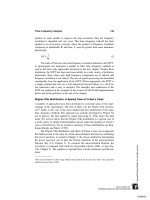
F
IGURE
11.4A MRI image of the brain before and after application of two filters
from MATLAB’s

fspecial
routine. Upper right: Image sharpening using the filter
unsharp
. Lower images: Edge detection using the
sobel
filter for horizontal
edges (left) and for both horizontal and vertical edges (right). (Original image
from MATLAB. Image Processing Toolbox. Copyright 1993–2003, The Math
Works, Inc. Reprinted with permission.)
% 3 by 3 Sobel edge detector filters to enhance horizontal and
% vertical edges.
% Combine the two edge detected images
%
clear all; close all;
%
frame = 17; % Load MRI frame 17
[I(:,:,:,1), map ] = imread(’mri.tif’, frame);
TLFeBOOK
Filters, Transformations, and Registration 315
F
IGURE
11.4B Frequency characteristics of the unsharp and Sobel filters used
in Example 11.2.
if isempty(map) == 0 % Usual check and
I = ind2gray(I,map); % conversion if
% necessary.
else
I = im2double(I);
end
%

h_unsharp = fspecial(’unsharp’,.5); % Generate ‘unsharp’
I_unsharp = imfilter(I,h_unsharp); % filter coef. and
% apply
%
h_s = fspecial(’Sobel’); % Generate basic Sobel
% filter.
I_sobel_horin = imfilter(I,h_s); % Apply to enhance
I_sobel_vertical = imfilter(I,h_s’); % horizontal and
% vertical edges
%
% Combine by converting to binary and or-ing together
I_sobel_combined = im2bw(I_sobel_horin) *
im2bw(I_sobel_vertical);
%
subplot(2,2,1); imshow(I); % Plot the images
title(’Original’);
subplot(2,2,2); imshow(I_unsharp);
title(’Unsharp’);
subplot(2,2,3); imshow(I_sobel_horin);
TLFeBOOK
316 Chapter 11
title(’Horizontal Sobel’);
subplot(2,2,4); imshow(I_sobel_combined);
title(’Combined Image’); figure;
%
% Now plot the unsharp and Sobel filter frequency
% characteristics
F= fftshift(abs(fft2(h_unsharp,32,32)));
subplot(1,2,1); mesh(1:32,1:32,F);
title(’Unsharp Filter’); view([-37,15]);

%
F = fftshift(abs(fft2(h_s,32,32)));
subplot(1,2,2); mesh(1:32,1:32,F);
title(’Sobel Filter’); view([-37,15]);
The images produced by this example program are shown below along
with the frequency characteristics associated with the
‘unsharp’
and
‘sobel’
filter. Note that the
‘unsharp’
filter has the general frequency characteristics
of a highpass filter, that is, a positive slope with increasing spatial frequencies
(Figure 11.4B). The double peaks of the Sobel filter that produce edge enhance-
ment are evident in Figure 11.4B. Since this is a magnitude plot, both peaks
appear as positive.
In Example 11.3, routine
ftrans2
is used to construct two-dimensional
filters from one-dimensional FIR filters. Lowpass and highpass filters are con-
structed using the filter design routine
fir1
from Chapter 4. This routine gener-
ates filter coefficients based on the ideal rectangular window approach described
in that chapter. Example 11.3 also illustrates the use of an alternate padding
technique to reduce the edge effects caused by zero padding. Specifically, the
‘replicate’
option of
imfilter
is used to pad by repetition of the last (i.e.,

image boundary) pixel value. This eliminates the dark border produced by zero
padding, but the effect is subtle.
Example 11.3 Example of the application of standard one-dimensional
FIR filters extended to two dimensions. The blood cell images (
blood1.tif
)
are loaded and filtered using a 32 by 32 lowpass and highpass filter. The one-
dimensional filter is based on the rectangular window filter (Eq. (10), Chapter
4), and is generated by
fir.
It is then extended to two dimensions using
ftrans2.
% Example 11.3 and Figure 11.5A and B
% Linear filtering. Load the blood cell image
% Apply a 32nd order lowpass filter having a bandwidth of .125
% fs/2, and a highpass filter having the same order and band-
% width. Implement the lowpass filter using ‘imfilter’ with the
TLFeBOOK
Filters, Transformations, and Registration 317
F
IGURE
11.5A Image of blood cells before and after lowpass and highpass filter-
ing. The upper lowpass image (upper right) was filtered using zero padding,
which produces a slight black border around the image. Padding by extending
the edge pixel eliminates this problem (lower left). (Original Image reprinted with
permission from The Image Processing Handbook, 2nd edition. Copyright CRC
Press, Boca Raton, Florida.)
% zero padding (the default) and with replicated padding
% (extending the final pixels).
% Plot the filter characteristics of the high and low pass filters

%
% Load the image and transform if necessary
clear all; close all;
N = 32; % Filter order
w_lp = .125; % Lowpass cutoff frequency
TLFeBOOK
318 Chapter 11
F
IGURE
11.5B Frequency characteristics of the lowpass (left) and highpass (right)
filters used in Figure 11.5A.
w_hp = .125; % Highpass cutoff frequency
load image blood1.tif and convert as in Example
11.2
%
b = fir1(N,w_lp); % Generate the lowpass filter
h_lp = ftrans2(b); % Convert to 2-dimensions
I_lowpass = imfilter(I,h_lp); % and apply with,
% and without replication
I_lowpass_rep = imfilter (I,h_lp,’replicate’);
b = fir1(N,w_hp,’high’); % Repeat for highpass
h_hp = ftrans2(b);
I_highpass = imfilter(I, h_hp);
I_highpass = mat2gray(I_highpass);
%
plot the images and filter characteristics as in
Example 11.2
The figures produced by this program are shown below (Figure 11.5A and
B). Note that there is little difference between the image filtered using zero
padding and the one that uses extended (

‘replicate’
) padding. The highpass
filtered image shows a slight derivative-like characteristic that enhances edges.
In the plots of frequency characteristics, Figure 11.5B, the lowpass and highpass
filters appear to be circular, symmetrical, and near opposites.
The problem of aliasing due to downsampling was discussed above and
TLFeBOOK
Filters, Transformations, and Registration 319
demonstrated in Figure 11.1. Such problems could occur whenever an image is
displayed in a smaller size that will require fewer pixels, for example when the
size of an image is reduced during reshaping of a computer window. Lowpass
filtering can be, and is, used to prevent aliasing when an image is downsized.
In fact, MATLAB automatically performs lowpass filtering when downsizing
an image. Example 11.4 demonstrates the ability of lowpass filtering to reduce
aliasing when downsampling is performed.
Example 11.4 Use lowpass filtering to reduce aliasing due to downsam-
pling. Load the radial pattern (
‘testpat1.png’
) and downsample by a factor
of six as was done in Figure 11.1. In addition, downsample that image by the
same amount, but after it has been lowpass filtered. Plot the two downsampled
images side-by-side. Use a 32 by 32 FIR rectangular window lowpass filter. Set
the cutoff frequency to be as high as possible and still eliminate most of the
aliasing.
% Example 11.4 and Figure 11.6
% Example of the ability of lowpass filtering to reduce aliasing.
% Downsample the radial pattern with and without prior lowpass
% filtering.
% Use a cutoff frequency sufficient to reduce aliasing.
%

clear all; close all;
N = 32; % Filter order
w = .5; % Cutoff frequency (see text)
F
IGURE
11.6 Two images of the radial pattern shown in Figure 11.1 after down-
sampling by a factor of 6. The right-hand image was filtered by a lowpass filter
before downsampling.
TLFeBOOK
320 Chapter 11
dwn = 6; % Downsampling coefficient
b = fir1(N,w); % Generate the lowpass filter
h = ftrans2(b); % Convert to 2-dimensions
%
[Imap] = imread(’testpat1.png’); % Load image
I_lowpass = imfilter(I,h); % Lowpass filter image
[M,N] = size(I);
%
I = I(1:dwn:M,1:dwn:N); % Downsample unfiltered image
subplot (1,2,1); imshow(I); % and display
title(’No Filtering’);
% Downsample filtered image and display
I_lowass = I_lowpass(1:dwn: M,1:dwn:N);
subplot(1,2,2); imshow(I_lowpass);
title (’Lowpass Filtered’);
The lowpass cutoff frequency used in Example 11.5 was determined em-
pirically. Although the cutoff frequency was fairly high ( f
S
/4), this filter still
produced substantial reduction in aliasing in the downsampled image.

SPATIAL TRANSFORMATIONS
Several useful transformations take place entirely in the spatial domain. Such
transformations include image resizing, rotation, cropping, stretching, shearing,
and image projections. Spatial transformations perform a remapping of pixels
and often require some form of interpolation in addition to possible anti-aliasing.
The primary approach to anti-aliasing is lowpass filtering, as demonstrated
above. For interpolation, there are three methods popularly used in image pro-
cessing, and MATLAB supports all three. All three interpolation strategies use
the same basic approach: the interpolated pixel in the output image is the
weighted sum of pixels in the vicinity of the original pixel after transformation.
The methods differ primarily in how many neighbors are considered.
As mentioned above, spatial transforms involve a remapping of one set of
pixels (i.e., image) to another. In this regard, the original image can be consid-
ered as the input to the remapping process and the transformed image is the
output of this process. If images were continuous, then remapping would not
require interpolation, but the discrete nature of pixels usually necessitates re-
mapping.* The simplest interpolation method is the nearest neighbor method in
which the output pixel is assigned the value of the closest pixel in the trans-
formed image, Figure 11.7. If the transformed image is larger than the original
and involves more pixels, then a remapped input pixel may fall into two or
*A few transformations may not require interpolation such as rotation by 90 or 180 degrees.
TLFeBOOK
Filters, Transformations, and Registration 321
F
IGURE
11.7 A rotation transform using the nearest neighbor interpolation
method. Pixel values in the output image (solid grid) are assigned values from
the nearest pixel in the transformed input image (dashed grid).
more output pixels. In the bilinear interpolation method, the output pixel is the
weighted average of transformed pixels in the nearest 2 by 2 neighborhood, and

in bicubic interpolation the weighted average is taken over a 4 by 4 neighbor-
hood.
Computational complexity and accuracy increase with the number of pix-
els that are considered in the interpolation, so there is a trade-off between quality
and computational time. In MATLAB, the functions that require interpolation
have an optional argument that specifies the method. For most functions, the
default method is nearest neighbor. This method produces acceptable results on
all image classes and is the only method appropriate for indexed images. The
method is also the most appropriate for binary images. For RGB and intensity
image classes, the bilinear or bicubic interpolation method is recommended
since they lead to better results.
MATLAB provides several routines that can be used to generate a variety
of complex spatial transformations such as image projections or specialized dis-
tortions. These transformations can be particularly useful when trying to overlay
(register) images of the same structure taken at different times or with different
modalities (e.g., PET scans and MRI images). While MATLAB’s spatial trans-
formations routines allow for any imaginable transformation, only two types
of transformation will be discussed here: affine transformations and projective
transformations. Affine transformations are defined as transformations in which
straight lines remain straight and parallel lines remain parallel, but rectangles
may become parallelograms. These transformations include rotation, scaling,
stretching, and shearing. In projective translations, straight lines still remain
straight, but parallel lines often converge toward vanishing points. These trans-
formations are discussed in the following MATLAB implementation section.
TLFeBOOK
322 Chapter 11
MATLAB Implementation
Affine Transformations
MATLAB provides a procedure described below for implementing any affine
transformation; however, some of these transformations are so popular they are

supported by separate routines. These include image resizing, cropping, and
rotation. Image resizing and cropping are both techniques to change the dimen-
sions of an image: the latter is interactive using the mouse and display while
the former is under program control. To change the size of an image, MATLAB
provides the
‘imresize’
command given below.
I_resize = imresize(I, arg or [M N], method);
where
I
is the original image and
I_resize
is the resized image. If the second
argument is a scalar arg, then it gives a magnification factor, and if it is a vector,
[M N]
, it indicates the desired new dimensions in vertical and horizontal pixels,
M, N.If
arg
> 1, then the image is increased (magnified) in size proportionally
and if
arg
< 1, it is reduced in size (minified). This will change image size
proportionally. If the vector
[M N]
is used to specify the output size, image
proportions can be modified: the image can be stretched or compressed along a
given dimension. The argument method specifies the type of interpolation to be
used and can be either
‘nearest’
,

‘bilinear’
,or
‘bicubic’
, referring to the
three interpolation methods described above. The nearest neighbor (
nearest
)is
the default. If image size is reduced, then
imresize
automatically applies an
anti- aliasing, lowpass filter unless the interpolation method is
nearest
; i.e., the
default. The logic of this is that the nearest neighbor interpolation method would
usually only be used with indexed images, and lowpass filtering is not really
appropriate for these images.
Image cropping is an interactive command:
I_resize = imcrop;
The
imcrop
routine waits for the operator to draw an on-screen cropping
rectangle using the mouse. The current image is resized to include only the
image within the rectangle.
Image rotation is straightforward using the
imrotate
command:
I_rotate = imrotate(I, deg, method, bbox);
where
I
is the input image,

I_rotate
is the rotated image,
deg
is the degrees
of rotation (counterclockwise if positive, and clockwise if negative), and
method
describes the interpolation method as in
imresize
. Again, the nearest neighbor
TLFeBOOK
Filters, Transformations, and Registration 323
method is the default even though the other methods are preferred except for
indexed images. After rotation, the image will not, in general, fit into the same
rectangular boundary as the original image. In this situation, the rotated image
can be cropped to fit within the original boundaries or the image size can be
increased to fit the rotated image. Specifying the
bbox
argument as
‘crop’
will
produce a cropped image having the dimensions of the original image, while
setting
bbox
to
‘loose’
will produce a larger image that contains the entire
original, unrotated, image. The
loose
option is the default. In either case, addi-
tional pixels will be required to fit the rotated image into a rectangular space

(except for orthogonal rotations), and
imrotate
pads these with zeros produc-
ing a black background to the rotated image (see Figure 11.8).
Application of the
imresize
and
imrotate
routines is shown in Example
11.5 below. Application of
imcrop
is presented in one of the problems at the
end of this chapter.
F
IGURE
11.8 Two spatial transformations (horizontal stretching and rotation) ap-
plied to an image of bone marrow. The rotated images are cropped either to
include the full image (lower left), or to have the same dimensions are the original
image (lower right). Stained image courtesy of Alan W. Partin, M.D., Ph.D., Johns
Hopkins University School of Medicine.
TLFeBOOK
324 Chapter 11
Example 11.5 Demonstrate resizing and rotation spatial transformat ions.
Load the i mage of stai ned tissue (
hestain.png
) and trans form it so that the
horizontal dimension is 25% longer than in the original, keeping the vertical di-
mension unchanged. Rotate the origina l image 45 degrees clock wise, with and
without cropping. Display the original and transformed images in a single figure.
% Example 11.5 and Figure 11.8

% Example of various Spatial Transformations
% Input the image of bone marrow (bonemarr.tif) and perform
% two spatial transformations:
% 1) Stretch the object by 25% in the horizontal direction;
% 2) Rotate the image clockwise by 30 deg. with and without
% cropping.
% Display the original and transformed images.
%
read image and convert if necessary
%
% Rotate image with and without cropping
I_rotate = imrotate(I,-45, ’bilinear’);
I_rotate_crop = imrotate (I, -45, ’bilinear’, ’crop’);
%
[M N] = size(I);
% Stretch by 25% horin.
I_stretch = imresize (I,[M N*1.25], ’bilinear’);
%
display the images
The images produced by this code are shown in Figure 11.8.
General Affine Transformations
In the MATLAB Image Processing Toolbox, both affine and projective spatial
transformations are defined by a
Tform
structure which is constructed using one
of two routines: the routine
maketform
uses parameters supplied by the user to
construct the transformation while
cp2tform

uses control points, or landmarks,
placed on different images to generate the transformation. Both routines are
very flexible and powerful, but that also means they are quite involved. This
section describes aspects of the
maketform
routine, while the
cp2tfrom
routine
will be presented in context with image registration.
Irrespective of the way in which the desired transformation is specified, it
is implemented using the routine
imtransform.
This routine is only slightly
less complicated than the transformation specification routines, and only some
of its features will be discussed here. (The associated help file should be con-
sulted for more detail.) The basic calling structure used to implement the spatial
transformation is:
TLFeBOOK
Filters, Transformations, and Registration 325
B = imtransform(A, Tform, ‘Param1’, value1, ‘Param2’,
value2, );
where
A
and
B
are the input and output arrays, respectively, and
Tform
provides
the transformation specifications as generated by
maketform

or
cp2tform.
The
additional arguments are optional. The optional parameters are specified as pairs
of arguments: a string containing the name of the optional parameter (i.e.,
‘Param1’
) followed by the value.* These parameters can (1) specify the pixels
to be used from the input image (the default is the entire image), (2) permit a
change in pixel size, (3) specify how to fill any extra background pixels gener-
ated by the transformation, and (4) specify the size and range of the output
array. Only the parameters that specify output range will be discussed here, as
they can be used to override the automatic rescaling of image size performed
by
imtransform
. To specify output image range and size, parameters
‘XData’
and
‘YData’
are followed by a two-variable vector that gives the x or y coordi-
nates of the first and last elements of the output array,
B
. To keep the size and
range in the output image the same as the input image, simply specify the hori-
zontal and vertical size of the input array, i.e.:
[M N] = size(A);

B = imtransform(A, Tform, ‘Xdata’, [1 N], ‘Ydata’, [1 M]);
As with the transform specification routines,
imtransform
uses the spa-

tial coordinate system described at the beginning of the Chapter 10. In this
system, the first dimension is the x coordinate while the second is the y,the
reverse of the matrix subscripting convention used by MATLAB. (However the
y coordinate still increases in the downward direction.) In addition, non-integer
values for x and y indexes are allowed.
The routine
maketform
can be used to generate the spatial transformation
descriptor,
Tform
. There are two alternative approaches to specifying the trans-
formation, but the most straightforward uses simple geometrical objects to de-
fine the transformation. The calling structure under this approach is:
Tform = maketform(‘type’, U, X);
where
‘type’
defines the type of transformation and
U
and
X
are vectors that
define the specific transformation by defining the input (
U
) and output (
X
) geom-
etries. While
maketform
supports a variety of transformation types, including
*This is a common approach used in many MATLAB routines when a large number of arguments

are possible, especially when many of these arguments are optional. It allows the arguments to be
specified in any order.
TLFeBOOK
326 Chapter 11
custom, user-defined types, only the affine and projective transformations will
be discussed here. These are specified by the
type
parameters
‘affine’
and
‘projective’
.
Only three points are required to define an affine transformation, so, for
this transformation type, U and X define corresponding vertices of input and
output triangles. Specifically, U and X are 3 by 2 matrices where each 2-column
row defines a corresponding vertex that maps input to output geometry. For
example, to stretch an image vertically, define an output triangle that is taller
than the input triangle. Assuming an input image of size M by N, to increase
the vertical dimension by 50% define input (
U
) and output (
X
) triangles as:
U = [1, 1; 1, M; N, M]’ X = [1, 1 5M; 1, M; N, M];
In this example, the input triangle,
U
, is simply the upper left, lower left,
and lower right corners of the image. The output triangle,
X
, has its top, left

vertex increased by 50%. (Recall the coordinate pairs are given as x,y and y
increases negatively. Note that negative coordinates are acceptable). To increase
the vertical dimension symmetrically, change
X
to:
X = [1, 1 25M; 1, 1.25*M; N, 1.25*M];
In this case, the upper vertex is increased by only 25%, and the two lower
vertexes are lowered in the y direction by increasing the y coordinate value by
25%. This transformation could be done with
imresize
, but this would also
change the dimension of the output image. When this transform is implemented
with
imtransform
, it is possible to control output size as described below.
Hence this approach, although more complicated, allows greater control of the
transformation. Of course, if output image size is kept the same, the contents of
the original image, when stretched, may exceed the boundaries of the image and
will be lost. An example of the use of this approach to change image proportions
is given in Problem 6.
The
maketform
routine can be used to implement other affine transforma-
tions such as shearing. For example, to shear an image to the left, define an
output triangle that is skewed by the desired amount with respect to the input
triangle, Figure 11.9. In Figure 11.9, the input triangle is specified as:
U = [N/
21;1M;NM]
, (solid line) and the output triangle as
X = [1 1; 1 M; N M]

(solid
line). This shearing transform is implemented in Example 11.6.
Projective Transformations
In projective transformations, straight lines remain straight but parallel lines
may converge. Projective transformations can be used to give objects perspec-
tive. Projective transformations require four points for definition; hence, the
TLFeBOOK
Filters, Transformations, and Registration 327
F
IGURE
11.9 An affine transformation can be defined by three points. The trans-
formation shown here is defined by an input (left) and output (right) triangle and
produces a sheared image. M,N are indicated in this figure as row, column, but
are actually specified in the algorithm in reverse order, as x,y. (Original image
from the MATLAB Image Processing Toolbox. Copyright 1993–2003, The Math
Work, Inc. Reprinted with permission.)
defining geometrical objects are quadrilaterals. Figure 11.10 shows a projective
transformation in which the original image would appear to be tilted back. In
this transformation, vertical lines in the original image would converge in the
transformed image. In addition to adding perspective, these transformations are
of value in correcting for relative tilts between image planes during image regis-
tration. In fact, most of these spatial transformations will be revisited in the
section on image registration. Example 11.6 illustrates the use of these general
image transformations for affine and projective transformations.
Example 11.6 General spatial transformations. Apply the affine and pro-
jective spatial transformation to one frame of the MRI image in
mri.tif
. The
affine transformation should skew the top of the image to the left, just as shown
in Figure 11.9. The projective transformation should tilt the image back as

shown in Figure 11.10. This example will also use projective transformation to
tilt the image forward, or opposite to that shown in Figure 11.10.
After the image is loaded, the affine input triangle is defined as an equilat-
eral triangle inscribed within the full image. The output triangle is defined by
shifting the top point to the left side, so the output triangle is now a right triangle
(see Figure 11.9). In the projective transformation, the input quadrilateral is a
TLFeBOOK
328 Chapter 11
F
IGURE
11.10 Specification of a projective transformation by defining two quadri-
laterals. The solid lines define the input quadrilateral and the dashed line defines
the desired output quadrilateral.
rectangle the same size as the input image. The output quadrilateral is generated
by moving the upper po ints inward and down by a n equal amount while the lower
points are moved outward and up, also by a fixed amount. The second projective
transformatio n is achieved by reversing the operations performed on the corners.
% Example 11.6 General Spatial Transformations
% Load a frame of the MRI image (mri.tif)
% and perform two spatial transformations
% 1) An affine transformation that shears the image to the left
% 2) A projective transformation that tilts the image backward
% 3) A projective transformation that tilts the image forward
clear all; close all;
%
% load frame 18
%
% Define affine transformation
U1 = [N/2 1; 1 M; N M]; % Input triangle
X1 = [1 1; 1 M; N M]; % Output triangle

% Generate transform
Tform1 = maketform(’affine’, U1, X1);
% Apply transform
I_affine = imtransform(I, Tform1,’Size’, [M N]);
%
% Define projective transformation vectors
offset = .25*N;
U = [1 1; 1 M; N M; N 1]; % Input quadrilateral
TLFeBOOK
Filters, Transformations, and Registration 329
X = [1-offset 1؉offset; 1؉offset M-offset;
N-offset M-offset; N؉offset 1؉offset];
%
% Define transformation based on vectors U and X
Tform2 = maketform(’projective’, U, X);
I_proj1 = imtransform(I,Tform2,’Xdata’,[1 N],’Ydata’,
[1 M]);
%
% Second transformation. Define new output quadrilateral
X = [1؉offset 1؉offset; 1-offset M-offset;
N؉offset M-offset; N-offset 1؉offset];
% Generate transform
Tform3 = maketform(’projective’, U, X);
% Apply transform
I_proj2 = imtransform(I,Tform3, ’Xdata’,[1 N],
’Ydata’,[1 M]);
%
display images
The images produced by this code are shown in Figure 11.11.
Of course, a great many other transforms can be constructed by redefining

the output (or input) triangles or quadrilaterals. Some of these alternative trans-
formations are explored in the problems.
All of these transforms can be applied to produce a series of images hav-
ing slightly different projections. When these multiple images are shown as a
movie, they will give an object the appearance of moving through space, per-
haps in three dimensions. The last three problems at the end of this chapter
explore these features. The following example demonstrates the construction of
such a movie.
Example 11.7 Construct a series of projective transformations, that
when shown as a movie, give the appearance of the image tilting backward in
space. Use one of the frames of the MRI image.
Solution The code below uses the projective transformation to generate
a series of images that appear to tilt back because of the geometry used. The
approach is based on the second projective transformation in Example 11.7, but
adjusts the transformation to produce a slightly larger apparent tilt in each
frame. The program fills 24 frames in such a way that the first 12 have increas-
ing angles of tilt and the last 12 frames have decreasing tilt. When shown as a
movie, the image will appear to rock backward and forward. This same ap-
proach will also be used in Problem 7. Note that as the images are being gener-
ated by
imtransform
, they are converted to indexed images using
gray2ind
since this is the format required by
immovie
. The grayscale map generated by
gray2ind
is used (at the default level of 64), but any other map could be
substituted in
immovie

to produce a pseudocolor image.
TLFeBOOK
330 Chapter 11
F
IGURE
11.11 Original MR image and three spatial transformations. Upper right:
An affine transformation that shears the image to the left. Lower left: A projective
transform in which the image is made to appear tilted forward. Lower right: A
projective transformation in which the image is made to appear tilted backward.
(Original image from the MATLAB Image Processing Toolbox, Copyright 1993–
2003, The Math Works, Inc. Reprinted with permission.)
% Example 11.7 Spatial Transformation movie
% Load a frame of the MRI image (mri.tif). Use the projective
% transformation to make a movie of the image as it tilts
% horizontally.
%
clear all; close all;
Nu_frame = 12; % Number of frames in each direction
Max_tilt = .5; % Maximum tilt achieved
load MRI frame 12 as in previous examples
TLFeBOOK
Filters, Transformations, and Registration 331
%
U = [1 1; 1 M; N M; N 1]; % Input quadrilateral
for i = 1:Nu_frame % Construct Nu_frame * 2 movie frames
% Define projective transformation Vary offset up to Max_tilt
offset = Max_tilt*N*i/Nu_frame;
X = [1؉offset 1؉offset; 1-offset M-offset; N؉offset
M-offset; N-offset 1؉offset];
Tform2 = maketform(’projective’, U, X);

[I_proj(:,:,1,i), map] = gray2ind(imtransform(I,Tform2,
’Xdata’,[1 N],’Ydata’,[1 M]));
% Make image tilt back and forth
I_proj(:,:,1,2*Nu_frame؉1-i) = I_proj(:,:,1,i);
end
%
% Display first 12 images as a montage
montage(I_proj(:,:,:,1:12),map);
mov = immovie(I_proj,map); % Display as movie
movie(mov,5);
While it is not possible to show the movie that is produced by this code,
the various frames are shown as a montage in Figure 11.12. The last three
problems in the problem set explore the use of spatial transformations used in
combination to make movies.
IMAGE REGISTRATION
Image registration is the alignment of two or more images so they best superim-
pose. This task has become increasingly important in medical imaging as it is
used for merging images acquired using different modalities (for example, MRI
and PET). Registration is also useful for comparing images taken of the same
structure at different points in time. In functional magnetic resonance imaging
(fMRI), image alignment is needed for images taken sequentially in time as
well as between images that have different resolutions. To achieve the best
alignment, it may be necessary to transform the images using any or all of the
transfo rm ati on s described previous ly. Image regi str at ion can be quite challen gin g
even when the images ar e identic al or ver y similar (as will be the case in the
example s and problems given here). Freq uen tl y the images to be aligne d are not
that similar, perha ps because the y have been acquir ed using differ en t modalities.
The difficult y in accurat el y alig nin g images tha t are only moderately similar pres-
ents a significant challe ng e to image registrati on algor ith ms, so the task is o ft en
aided by a human intervent io n or the use of embedde d markers for refere nce .

Approaches to image registration can be divided into two broad catego-
ries: unassisted image registration where the algorithm generates the alignment
without human intervention, and interactive registration where a human operator
TLFeBOOK
332 Chapter 11
F
IGURE
11.12 Montage display of the movie produced by the code in Example
11.7. The various projections give the appearance of the brain slice tilting and
moving back in space. Only half the 24 frames are shown here as the rest are
the same, just presented in reverse order to give the appearance of the brain
rocking back and forth. (Original image from the MATLAB Image Processing
Toolbox. Copyright 1993–2003, The Math Works, Inc. Reprinted with permis-
sion.)
TLFeBOOK
Filters, Transformations, and Registration 333
guides or aids the registration process. The former approach usually relies on
some optimization technique to maximize the correlation between the images.
In the latter approach, a human operator may aid the alignment process by
selecting corresponding reference points in the images to be aligned: corre-
sponding features are identified by the operator and tagged using some interac-
tive graphics procedure. This approach is well supported in MATLAB’s Image
Processing Toolbox. Both of these approaches are demonstrated in the examples
and problems.
Unaided Image Registration
Unaided image registration usually involves the application of an optimization
algorithm to maximize the correlation, or other measure of similarity, between
the images. In this strategy, the appropriate transformation is applied to one of
the images, the input image, and a comparison is made between this transformed
image and the reference image (also termed the base image). The optimization

routine seeks to vary the transformation in some manner until the comparison
is best possible. The problem with this approach is the same as with all optimi-
zation techniques: the optimization process may converge on a sub-optimal solu-
tion (a so-called local maximum), not the optimal solution (the global maxi-
mum). Often the solution achieved depends on the starting values of the
transformation variables. An example of convergence to a sub-optimal solution
and dependency on initial variables is found in Problem 8.
Example 11.8 below uses the optimization routine that is part of the basic
MATLAB package,
fminsearch
(formerly
fmins
). This routine is based on the
simplex (direct search) method, and will adjust any number of parameters to
minimize a function specified though a user routine. To maximize the correspon-
dence between the reference image and the input image, the negative of the
correlation between the two images is minimized. The routine
fminsearch
will
automatically adjust the transformation variables to achieve this minimum (re-
member that this may not be the absolute minimum).
To implement an optimization search, a routine is required that applies
the transformation variables supplied by
fminsearch
, performs an appropriate
trial transformation on the input image, then compares the trial image with the
reference image. Following convergence, the optimization routine returns the
values of the transformation variables that produce the best comparison. These
can then be applied to produce the final aligned image. Note that the program-
mer must specify the actual structure of the transformation since the optimiza-

tion routine works blindly and simply seeks a set of variables that produces a
minimum output. The transformation selected should be based on the possible
mechanisms for misalignment: translations, size changes, rotations, skewness,
projective misalignment, or other more complex distortions. For efficiency, the
transformation should be one that requires the least number of defining vari-
TLFeBOOK
334 Chapter 11
ables. Reducing the number of variables increases the likelihood of optimal
convergence and substantially reduces computation time. To minimize the num-
ber of transformation variables, the simplest transformation that will compensate
for the possible mechanisms of distortions should be used.*
Example 11.8 This is an example of unaided image registration requir-
ing an affine transformation. The input image, the image to be aligned, is a
distorted version of the reference image. Specifically, it has been stretched hori-
zontally, compressed vertically, and tilted, all using a single affine transforma-
tion. The problem is to find a transformation that will realign this image with
the reference image.
Solution MATLAB’s optimization routine
fminsearch
will be used to
determine an optimized transformation that will make the two images as similar
as possible. MATLAB’s
fminsearch
routine calls the user routine
rescale
to
perform the transformation and make the comparison between the two images.
The
rescale
routine assumes that an affine transformation is required and that

only the horizontal, vertical, and tilt dimensions need to be adjusted. (It does
not, for exampl e, take into account possible translations between the two images,
although this would not be too difficult to incorporate.) The
fminsearch
routine
requires as input arguments, the name of the routine whose output is to be mini-
mized (in this example,
rescale
), and the initial values of the transformation
variables (in this example, all 1’s). The routine uses the size of the initial value
vector to determine how many variables it needs to adjust (in this case, three
variables). Any additional input arguments following an optional vector specify-
ing operational features are passed to
rescale
immediately following the trans-
formation variables. The optimization routine will continue to call
rescale
au-
tomatically until it has found an acceptable minimum for the error (or until
some maximum number of iterations is reached, see the associated help file).
% Example 11.8 and Figure 11.13
% Image registration after spatial transformation
% Load a frame of the MRI image (mri.tif). Transform the original
% image by increasing it horizontally, decreasing it vertically,
% and tilting it to the right. Also decrease image contrast
% slightly
% Use MATLAB’s basic optimization routine, ’fminsearch’ to find
% the transformation that restores the original image shape.
%
*The number of defining variables depends on the transformation. For example rotation alone only

requires one variable, linear transformations require two variables, affine transformations require 3
variables while projective transformations require 4 variables. Two additional variables are required
for translations.
TLFeBOOK
Filters, Transformations, and Registration 335
F
IGURE
11.13 Unaided image registration requiring several affine transforma-
tions. The left image is the original (reference) image and the distorted center
image is to be aligned with that image. After a transformation determined by opti-
mization, the right image is quite similar to the reference image. (Original image
from the same as fig 11.12.)
clear all; close all;
H_scale = .25; % Define distorting parameters
V_scale = .2; % Horizontal, vertical, and tilt
tilt = .2; % in percent
load mri.tif, frame 18
[M N]= size(I);
H_scale = H_scale * N/2; % Convert percent scale to pixels
V_scale = V_scale * M;
tilt = tilt * N
%
% Construct distorted image.
U = [1 1; 1 M; N M]; % Input triangle
X = [1-H_scale؉tilt 1؉V_scale; 1-H_scale M; N؉H_scale M];
Tform = maketform(’affine’, U, X);
I_transform = (imtransform(I,Tform,’Xdata’,[1 N],
’Ydata’, [1 M]))*.8;
%
% Now find transformation to realign image

initial_scale = [1 1 1]; % Set initial values
[scale,Fval] = fminsearch(’rescale’,initial_scale,[ ],
I, I_transform);
disp(Fval) % Display final correlation
%
% Realign image using optimized transform
TLFeBOOK