Biosignal and Biomedical Image Processing MATLAB-Based Applications Muya phần 7 potx

222 Chapter 8
%
% Plot frequency characteristics of unknown and identified
% process
f = (1:N) * fs/N; % Construct freq. vector for
% plotting
subplot(1,2,1); % Plot unknown system freq. char.
plot(f(1:N/2),ps_unknown(1:N/2),’k’);
labels, table, axis
subplot(1,2,2);
% Plot matching system freq. char.
plot(f(1:N/2),ps_match(1:N/2),’k’);
labels, table, axis
The output plots from this example are shown in Figure 8.4. Note the
close match in spectral characteristics between the “unknown” process and the
matching output produced by the Wiener-Hopf algorithm. The transfer functions
also closely match as seen by the similarity in impulse response coefficients:
h(n)
unknown
= [0.5 0.75 1.2]; h(n)
match
= [0.503 0.757 1.216].
ADAPTIVE SIGNAL PROCESSING
The area of adaptive signal processing is relatively new yet already has a rich
history. As with optimal filtering, only a brief example of the usefulness and
broad applicability of adaptive filtering can be covered here. The FIR and IIR
filters described in Chapter 4 were based on an a priori design criteria and were
fixed throughout their application. Although the Wiener filter described above
does not require prior knowledge of the input signal (only the desired outcome),
it too is fixed for a given application. As with classical spectral analysis meth-
ods, these filters cannot respond to changes that might occur during the course

of the signal. Adaptive filters have the capability of modifying their properties
based on selected features of signal being analyzed.
A typical adaptive filter paradigm is shown in Figure 8.5. In this case, the
filter co effic ients are modified by a feedback process designed to make the filter’s
output, y(n), as close to some desired response, d(n), as possible, by reducing the
error, e(n), to a minimum. As with optim al filtering, the nature of the desi red
response will depend on the specific problem involved and its formulation may
be the most diff icult part o f the a dapti ve sys tem sp ecification (Stearns and David,
1996).
The inherent stabili ty of FIR fil ters makes t hem attract ive in adapt ive ap pli-
cations as well as in optimal filtering (Ingle and Proakis, 2000). Accordingly, the
adaptive filter, H(z), can again be represented by a set of FIR filter coefficients,
TLFeBOOK
Advanced Signal Processing 223
F
IGURE
8.5 Elements of a typical adaptive filter.
b(k). The FIR filter equation (i.e., convolution) is repeated here, but the filter
coefficients are indicated as b
n
(k) to indicate that they vary with time (i.e., n).
y(n) =
∑
L
k=1
b
n
(k) x(n − k)(8)
The adaptive filter operates by modifying the filter coefficients, b
n

(k),
based on some signal property. The general adaptive filter problem has similari-
ties to the Wiener filter theory problem discussed above in that an error is
minimized, usually between the input and some desired response. As with opti-
mal filtering, it is the squared error that is minimized, and, again, it is necessary
to somehow construct a desired signal. In the Wiener approach, the analysis is
applied to the entire waveform and the resultant optimal filter coefficients were
similarly applied to the entire waveform (a so-called block approach). In adap-
tive filtering, the filter coefficients are adjusted and applied in an ongoing basis.
While the Wiener-Hopf equ at ion s (Eqs. (6) and (7)) can be, and have been,
adapted for use in an adaptive environment, a simpler and more popular ap-
proach is based on gradient optimization. This approach is usually called the
LMS recursive algorithm. As in Wiener filter theory, this algorithm also deter-
mines the optimal filter coefficients, and it is also based on minimizing the
squared error, but it does not require computation of the correlation functions,
r
xx
and r
xy
. Instead the LMS algorithm uses a recursive gradient method known
as the steepest-descent method for finding the filter coefficients that produce
the minimum sum of squared error.
Examination of Eq. (3) shows that the sum of squared errors is a quadratic
function of the FIR filter coefficients, b(k); hence, this function will have a
single minimum. The goal of the LMS algorithm is to adjust the coefficients so
that the sum of squared error moves toward this minimum. The technique used
by the LMS algorithm is to adjust the filter coefficients based on the method of
steepest descent. In this approach, the filter coefficients are modified based on
TLFeBOOK
224 Chapter 8

an estimate of the negative gradient of the error function with respect to a given
b(k). This estimate is given by the partial derivative of the squared error, ε, with
respect to the coefficients, b
n
(k):
᭞
n
=
∂ε
n
2
∂b
n
(k)
= 2e(n)
∂(d(n) − y(n))
∂b
n
(k)
(9)
Since d(n) is independent of the coefficients, b
n
(k), its partial derivative
with respect to b
n
(k) is zero. As y(n) is a function of the input times b
n
(k) (Eq.
(8)), then its partial derivative with respect to b
n

(k) is just x(n-k), and Eq. (9)
can be rewritten in terms of the instantaneous product of error and the input:
᭞
n
= 2e(n) x(n − k)(10)
Initially, the filter coefficients are set arbitrarily to some b
0
(k), usually
zero. With each new input sample a new error signal, e(n), can be computed
(Figure 8.5). Based on this new error signal, the new gradient is determined
(Eq. (10)), and the filter coefficients are updated:
b
n
(k) = b
n−1
(k) +∆e(n) x(n − k)(11)
where ∆ is a constant that controls the descent and, hence, the rate of conver-
gence. This parameter must be chosen with some care. A large value of ∆ will
lead to large modifications of the filter coefficients which will hasten conver-
gence, but can also lead to instability and oscillations. Conversely, a small value
will result in slow convergence of the filter coefficients to their optimal values.
A common rule is to select the convergence parameter, ∆, such that it lies in
the range:
0 <∆<
1
10LP
x
(12)
where L is the length of the FIR filter and P
x

is the power in the input signal.
P
X
can be approximated by:
P
x
Ϸ
1
N − 1
∑
N
n=1
x
2
(n)(13)
Note that for a waveform of zero mean, P
x
equals the variance of x. The
LMS algorithm given in Eq. (11) can easily be implemented in MATLAB, as
shown in the next section.
Adaptive filtering has a number of applications in biosignal processing. It
can be used to suppress a narrowband noise source such as 60 Hz that is corrupt-
ing a broadband signal. It can also be used in the reverse situation, removing
broadband noise from a narrowband signal, a process known as adaptive line
TLFeBOOK
Advanced Signal Processing 225
F
IGURE
8.6 Configuration for Adaptive Line Enhancement (ALE) or Adaptive In-
terference Suppression. The Delay, D, decorrelates the narrowband component

allowing the adaptive filter to use only this component. In ALE the narrowband
component is the signal while in Interference suppression it is the noise.
enhancement (ALE).* It can also be used for some of the same applications
as the Wiener filter such as system identification, inverse modeling, and, espe-
cially important in biosignal processing, adaptive noise cancellation. This last
application requires a suitable reference source that is correlated with the noise,
but not the signal. Many of these applications are explored in the next section
on MATLAB implementation and/or in the problems.
The configuration for ALE and adaptive interference suppression is shown
in Figure 8.6. When this configuration is used in adaptive interference suppres-
sion, the input consists of a broadband signal, Bb(n), in narrowband noise,
Nb(n), such as 60 Hz. Since the noise is narrowband compared to the relatively
broadband signal, the noise portion of sequential samples will remain correlated
while the broadband signal components will be decorrelated after a few sam-
ples.† If the combined signal and noise is delayed by D samples, the broadband
(signal) component of the delayed waveform will no longer be correlated with
the broadband component in the original waveform. Hence, when the filter’s
output is subtracted from the input waveform, only the narrowband component
*The adaptive line enhancer is so termed because the objective of this filter is to enhance a narrow-
band signal, one with a spectrum composed of a single “line.”
†Recall that the width of the autocorrelation function is a measure of the range of samples for which
the samples are correlated, and this width is inversely related to the signal bandwidth. Hence, broad-
band signals remain correlated for only a few samples and vice versa.
TLFeBOOK
226 Chapter 8
can have an influence on the result. The adaptive filter will try to adjust its
output to minimize this result, but since its output component, Nb *(n), only
correlates with the narrowband component of the waveform, Nb(n), it is only
the narrowband component that is minimized. In adaptive interference suppres-
sion, the narrowband component is the noise and this is the component that is

minimized in the subtracted signal. The subtracted signal, now containing less
noise, constitutes the output in adaptive interference suppression (upper output,
Figure 8.6).
In adaptive line enhancement, the configuration is the same except the
roles of signal and noise are reversed: the narrowband component is the signal
and the broadband component is the noise. In this case, the output is taken from
the filter output (Figure 8.6, lower output). Recall that this filter output is opti-
mized for the narrowband component of the waveform.
As with the Wiener filter approach, a filter of equal or better performance
could be constructed with the same number of filter coefficients using the tradi-
tional methods described in Chapter 4. However, the exact frequency or frequen-
cies of the signal would have to be known in advance and these spectral features
would have to be fixed throughout the signal, a situation that is often violated
in biological signals. The ALE can be regarded as a self-tuning narrowband
filter which will track changes in signal frequency. An application of ALE is
provided in Example 8.3 and an example of adaptive interference suppression
is given in the problems.
Adaptive Noise Cancellation
Adaptive noise cancellation can be thought of as an outgrowth of the interfer-
ence suppression described above, except that a separate channel is used to
supply the estimated noise or interference signal. One of the earliest applications
of adaptive noise cancellation was to eliminate 60 Hz noise from an ECG signal
(Widrow, 1964). It has also been used to improve measurements of the fetal
ECG by reducing interference from the mother’s EEG. In this approach, a refer-
ence channel carries a signal that is correlated with the interference, but not
with the signal of interest. The adaptive noise canceller consists of an adaptive
filter that operates on the reference signal, N’(n), to produce an estimate of the
interference, N(n) (Figure 8.7). This estimated noise is then subtracted from the
signal channel to produce the output. As with ALE and interference cancella-
tion, the difference signal is used to adjust the filter coefficients. Again, the

strategy is to minimize the difference signal, which in this case is also the
output, since minimum output signal power corresponds to minimum interfer-
ence, or noise. This is because the only way the filter can reduce the output
power is to reduce the noise component since this is the only signal component
available to the filter.
TLFeBOOK
Advanced Signal Processing 227
F
IGURE
8.7 Configuration for adaptive noise cancellation. The reference channel
carries a signal, N’(n), that is correlated with the noise, N(n), but not with the
signal of interest, x(n). The adaptive filter produces an estimate of the noise,
N*(n), that is in the signal. In some applications, multiple reference channels are
used to provide a more accurate representation of the background noise.
MATLAB Implementation
The implementation of the LMS recursive algorithm (Eq. (11)) in MATLAB is
straightforward and is given below. Its application is illustrated through several
examples below.
The LMS algorithm is implemented in the function
lms
.
function [b,y,e] = lms(x,d,delta,L)
%
% Inputs: x = input
%d= desired signal
% delta = the convergence gain
% L is the length (order) of the FIR filter
% Outputs: b = FIR filter coefficients
%y= ALE output
%e= residual error

% Simple function to adjust filter coefficients using the LSM
% algorithm
% Adjusts filter coefficients, b, to provide the best match
% between the input, x(n), and a desired waveform, d(n),
% Both waveforms must be the same length
% Uses a standard FIR filter
%
M = length(x);
b = zeros(1,L); y = zeros(1,M); % Initialize outputs
for n = L:M
TLFeBOOK
228 Chapter 8
x1 = x(n:-1:n-L؉1); % Select input for convolu-
% tion
y(n) = b * x1’; % Convolve (multiply)
% weights with input
e(n) = d(n)—y(n); % Calculate error
b = b ؉ delta*e(n)*x1; % Adjust weights
end
Note that this function operates on the data as block, but could easily be
modified to operate on-line, that is, as the data are being acquired. The routine
begins by applying the filter with the current coefficients to the first
L
points (
L
is the filter length), calculates the error between the filter output and the desired
output, then adjusts the filter coefficients accordingly. This process is repeated
for another data segment
L
-points long, beginning with the second point, and

continues through the input waveform.
Example 8.3 Optimal filtering using the LMS algorithm. Given the
same sinusoidal signal in noise as used in Example 8.1, design an adaptive filter
to remove the noise. Just as in Example 8.1, assume that you have a copy of
the desired signal.
Solution The program below sets up the problem as in Example 8.1, but
uses the LMS algorithm in the routine
lms
instead of the Wiener-Hopf equation.
% Example 8.3 and Figure 8.8 Adaptive Filters
% Use an adaptive filter to eliminate broadband noise from a
% narrowband signal
% Use LSM algorithm applied to the same data as Example 8.1
%
close all; clear all;
fs = 1000;*IH26* % Sampling frequency
N = 1024; % Number of points
L = 256; % Optimal filter order
a = .25; % Convergence gain
%
% Same initial lines as in Example 8.1
%% Calculate convergence parameter
PX = (1/(N؉1))* sum(xn.v2); % Calculate approx. power in xn
delta = a * (1/(10*L*PX)); % Calculate ⌬
b = lms(xn,x,delta,L); % Apply LMS algorithm (see below)
%
% Plotting identical to Example 8.1.
Example 8.3 produces the data in Figure 8.8. As with the Wiener filter,
the adaptive process adjusts the FIR filter coefficients to produce a narrowband
filter centered about the sinusoidal frequency. The convergence factor,

a
, was
TLFeBOOK
Advanced Signal Processing 229
F
IGURE
8.8 Application of an adaptive filter using the LSM recursive algorithm
to data containing a single sinusoid (10 Hz) in noise (SNR = -8 db). Note that the
filter requires the first 0.4 to 0.5 sec to adapt (400–500 points), and that the fre-
quency characteristics of the coefficients produced after adaptation are those of
a bandpass filter with a single peak at 10 Hz. Comparing this figure with Figure
8.3 suggests that the adaptive approach is somewhat more effective than the
Wiener filter for the same number of filter weights.
empirically set to give rapid, yet stable convergence. (In fact, close inspection of
Figure 8.8 shows a small oscillation in the output amplitude suggesting marginal
stability.)
Example 8.4 The application of the LMS algorithm to a stationary sig-
nal was given in Example 8.3. Example 8.4 explores the adaptive characteristics
of algorithm in the context of an adaptive line enhancement problem. Specifi-
cally, a single sinusoid that is buried in noise (SNR = -6 db) abruptly changes
frequency. The ALE-type filter must readjust its coefficients to adapt to the new
frequency.
The signal consists of two sequential sinusoids of 10 and 20 Hz, each
lasting 0.6 sec. An FIR filter with 256 coefficients will be used. Delay and
convergence gain will be set for best results. (As in many problems some adjust-
ments must be made on a trial and error basis.)
TLFeBOOK
230 Chapter 8
Solution Use the LSM recursive algorithm to implement the ALE filter.
% Example 8.4 and Figure 8.9 Adaptive Line Enhancement (ALE)

% Uses adaptive filter to eliminate broadband noise from a
% narrowband signal
%
% Generate signal and noise
close all; clear all;
fs = 1000; % Sampling frequency
F
IGURE
8.9 Adaptive line enhancer applied to a signal consisting of two sequen-
tial sinusoids having different frequencies (10 and 20 Hz). The delay of 5 samples
and the convergence gain of 0.075 were determined by trial and error to give the
best results with the specified FIR filter length.
TLFeBOOK
Advanced Signal Processing 231
L = 256; % Filter order
N = 2000; % Number of points
delay = 5; % Decorrelation delay
a = .075; % Convergence gain
t = (1:N)/fs; % Time vector for plotting
%
% Generate data: two sequential sinusoids, 10 & 20 Hz in noise
% (SNR = -6)
x = [sig_noise(10,-6,N/2) sig_noise(20,-6,N/2)];
%
subplot(2,1,1); % Plot unfiltered data
plot(t, x,’k’);
axis, title
PX = (1/(N؉1))* sum(x.v2); % Calculate waveform
% power for delta
delta = (1/(10*L*PX)) * a; % Use 10% of the max.

% range of delta
xd = [x(delay:N) zeros(1,delay-1)]; % Delay signal to decor-
% relate broadband noise
[b,y] = lms(xd,x,delta,L); % Apply LMS algorithm
subplot(2,1,2); % Plot filtered data
plot(t,y,’k’);
axis, title
The results of this code are shown in Figure 8.9. Several values of delay
were evaluated and the delay chosen, 5 samples, showed marginally better re-
sults than other delays. The convergence gain of 0.075 (7.5% maximum) was
also determined empirically. The influence of delay on ALE performance is
explored in Problem 4 at the end of this chapter.
Example 8.5 The application of the LMS algorithm to adaptive noise
cancellation is given in this example. Here a single sinusoid is considered as
noise and the approach reduces the noise produced the sinusoidal interference
signal. We assume that we have a scaled, but otherwise identical, copy of the
interference signal. In practice, the reference signal would be correlated with,
but not necessarily identical to, the interference signal. An example of this more
practical situation is given in Problem 5.
% Example 8.5 and Figure 8.10 Adaptive Noise Cancellation
% Use an adaptive filter to eliminate sinusoidal noise from a
% narrowband signal
%
% Generate signal and noise
close all; clear all;
TLFeBOOK
232 Chapter 8
F
IGURE
8.10 Example of adaptive noise cancellation. In this example the refer-

ence signal was simply a scaled copy of the sinusoidal interference, while in a
more practical situation the reference signal would be correlated with, but not
identical to, the interference. Note the near perfect cancellation of the interfer-
ence.
fs = 500; % Sampling frequency
L = 256; % Filter order
N = 2000; % Number of points
t = (1:N)/fs; % Time vector for plotting
a = 0.5; % Convergence gain (50%
% maximum)
%
% Generate triangle (i.e., sawtooth) waveform and plot
w = (1:N) * 4 * pi/fs; % Data frequency vector
x = sawtooth(w,.5); % Signal is a triangle
% (sawtooth)
TLFeBOOK
Advanced Signal Processing 233
subplot(3,1,1); plot(t,x,’k’); % Plot signal without noise
axis, title
% Add interference signal: a sinusoid
intefer = sin(w*2.33); % Interfer freq. = 2.33
% times signal freq.
x = x ؉ intefer; % Construct signal plus
% interference
ref = .45 * intefer; % Reference is simply a
% scaled copy of the
% interference signal
%
subplot(3,1,2); plot(t, x,’k’); % Plot unfiltered data
axis, title

%
% Apply adaptive filter and plot
Px = (1/(N؉1))* sum(x.v2); % Calculate waveform power
% for delta
delta = (1/(10*L*Px)) * a; % Convergence factor
[b,y,out] = lms(ref,x,delta,L); % Apply LMS algorithm
subplot(3,1,3); plot(t,out,’k’); % Plot filtered data
axis, title
Results in Figure 8.10 show very good cancellation of the sinusoidal inter-
ference signal. Note that the adaptation requires approximately 2.0 sec or 1000
samples.
PHASE SENSITIVE DETECTION
Phase sensitive detection, also known as synchronous detection, is a technique
for demodulating amplitude modulated (AM) signals that is also very effective
in reducing noise. From a frequency domain point of view, the effect of ampli-
tude modulation is to shift the signal frequencies to another portion of the spec-
trum; specifically, to a range on either side of the modulating, or “carrier,”
frequency. Amplitude modulation can be very effective in reducing noise be-
cause it can shift signal frequencies to spectral regions where noise is minimal.
The application of a narrowband filter centered about the new frequency range
(i.e., the carrier frequency) can then be used to remove the noise outside the
bandwidth of the effective bandpass filter, including noise that may have been
present in the original frequency range.*
Phase sensitive detection is most commonly implemented using analog
*Many biological signals contain frequencies around 60 Hz, a major noise frequency.
TLFeBOOK
234 Chapter 8
hardware. Prepackaged phase sensitive detectors that incorporate a wide variety
of optional features are commercially available, and are sold under the term
lock-in amplifiers. While lock-in amplifiers tend to be costly, less sophisticated

analog phase sensitive detectors can be constructed quite inexpensively. The
reason phase sensitive detection is commonly carried out in the analog domain
has to do with the limitations on digital storage and analog-to-digital conversion.
AM signals consist of a carrier signal (usually a sinusoid ) which has an ampli-
tude that is varied by the signal of interest. For this to work without loss of
information, the frequency of the carrier signal must be much higher than the
highest frequency in the signal of interest. (As with sampling, the greater the
spread between the highest signal frequency and the carrier frequency, the easier
it is to separate the two after demodulation.) Since sampling theory dictates that
the sampling frequency be at least twice the highest frequency in the input
signal, the sampling frequency of an AM signal must be more than twice the
carrier frequency. Thus, the sampling frequency will need to be much higher
than the highest frequency of interest, much higher than if the AM signal were
demodulated before sampling. Hence, digitizing an AM signal before demodula-
tion places a higher burden on memory storage requirements and analog-to-
digital conversion rates. However, with the reduction in cost of both memory
and highspeed ADC’s, it is becoming more and more practical to decode AM
signals using the software equivalent of phase sensitive detection. The following
analysis applies to both hardware and software PSD’s.
AM Modulation
In an AM signal, the amplitude of a sinusoidal carrier signal varies in proportion
to changes in the signal of interest. AM signals commonly arise in bioinstrumen-
tation systems when transducer based on variation in electrical properties is
excited by a sinusoidal voltage (i.e., the current through the transducer is sinus-
oidal). The strain gage is an example of this type of transducer where resistance
varies in proportion to small changes in length. Assume that two strain gages
are differential configured and connected in a bridge circuit, as shown in Figure
1.3. One arm of the bridge circuit contains the transducers, R +∆R and R −∆R,
while the other arm contains resistors having a fixed value of R, the nominal
resistance value of the strain gages. In this example, ∆R will be a function of

time, specifically a sinusoidal function of time, although in the general case it
would be a time varying signal containing a range of sinusoid frequencies. If
the bridge is balanced, and ∆R << R, then it is easy to show using basic circuit
analysis that the bridge output is:
V
in
=∆RV/2R (14)
TLFeBOOK
Advanced Signal Processing 235
where V is source voltage of the bridge. If this voltage is sinusoidal, V = V
s
cos
(ω
c
t), then V
in
(t) becomes:
V
in
(t) = (V
s
∆R/2R)cos(ω
c
t) (15)
If the input to the strain gages is sinusoidal, then ∆R = k cos(ω
s
t); where
ω
s
is the signal frequency and is assumed to be << ω

c
and k is the strain gage
sensitivity. Still assuming ∆R << R, the equation for V
in
(t) becomes:
V
in
(t) = V
s
k/2R [cos(ω
s
t)cos(ω
c
t)] (16)
Now applying the trigonometric identity for the product of two cosines:
cos(x)cos(y) =
1
2
cos(x + y) +
1
2
cos(x − y) (17)
the equation for V
in
(t) becomes:
V
in
(t) = V
s
k/4R [cos(ω

c
+ω
s
)t + cos(ω
c
−ω
s
)t] (18)
This signal would have the magnitude spectrum given in Figure 8.11. This
signal is termed a double side band suppressed-carrier modulation since the
carrier frequency, ω
c
, is missing as seen in Figure 8.11.
F
IGURE
8.11 Frequency spectrum of the signal created by sinusoidally exciting
a variable resistance transducer with a carrier frequency ω
c
. This type of modula-
tion is termed double sideband suppressed-carrier modulation since the carrier
frequency is absent.
TLFeBOOK
236 Chapter 8
Note that using the identity:
cos(x) + cos(y) = 2cos
ͩ
x + y
2
ͪ
cos

ͩ
x − y
2
ͪ
(19)
then V
in
(t) can be written as:
V
in
(t) = V
s
k/2R (cos(ω
c
t)cos(ω
s
t)) = A(t)cos(ω
c
t)(20)
where
A(t) = V
s
k/2R (cos(ω
cs
t)) (21)
Phase Sensitive Detectors
The basic configuration of a phase sensitive detector is shown in Figure 8.12
below. The first step in phase sensitive detection is multiplication by a phase
shifted carrier.
Using the identity given in Eq. (18) the output of the multiplier, V′(t), in

Figure 8.12 becomes:
V′(t) = V
in
(t)cos(ω
c
t +θ) = A(t)cos(ω
c
t) cos(ω
c
t +θ)
= A(t)/2 [cos(2ω
c
t +θ) + cos θ](22)
To get the full spectrum, before filtering, substitute Eq. (21) for A(t)into
Eq. (22):
V′(t) = V
s
k/4R [cos(2ω
c
t +θ)cos(ω
s
t) + cos(ω
s
t)cosθ)] (23)
again applying the identity in Eq. (17):
F
IGURE
8.12 Basic elements and configuration of a phase sensitive detector
used to demodulate AM signals.
TLFeBOOK

Advanced Signal Processing 237
V′(t) = V
s
k/4R [cos(2ω
c
t +θ+ω
s
t) + cos(2ω
c
t +θ−ω
s
t)
+ cos(ω
s
t +θ) + cos(ω
s
t −θ)] (24)
The spectrum of V ′(t) is shown in Figure 8.13. Note that the phase angle,
θ, would have an influence on the magnitude of the signal, but not its frequency.
After lowpass digital filtering the higher frequency terms, ω
c
t ±ω
s
will be
reduced to near zero, so the output, V
out
(t), becomes:
V
out
(t) = A(t)cosθ=(V

s
k/2R)cosθ (25)
Since cos θ is a constant, the output of the phase sensitive detector is the
demodulated signal, A(t), multiplied by this constant. The term phase sensitive
is derived from the fact that the constant is a function of the phase difference,
θ, between V
c
(t) and V
in
(t). Note that while θ is generally constant, any shift in
phase between the two signals will induce a change in the output signal level,
so this approach could also be used to detect phase changes between signals of
constant amplitude.
The multiplier operation is similar to the sampling process in that it gener-
ates additional frequency components. This will reduce the influence of low
frequency noise since it will be shifted up to near the carrier frequency. For
example, consider the effect of the multiplier on 60 Hz noise (or almost any
noise that is not near to the carrier frequency). Using the principle of superposit-
ion, only the noise component needs to be considered. For a noise component
at frequency, ω
n
(V
in
(t)
NOISE
= V
n
cos (ω
n
t)). After multiplication the contribution

at V′(t) will be:
F
IGURE
8.13 Frequency spectrum of the signal created by multiplying the V
in
(t)
by the carrier frequency. After lowpass filtering, only the original low frequency
signal at ω
s
will remain.
TLFeBOOK
238 Chapter 8
V
in
(t)
NOISE
= V
n
[cos(ω
c
t +ω
n
t) + cos(ω
c
t +ω
s
t)] (26)
and the new, complete spectrum for V′(t) is shown in Figure 8.14.
The only frequencies that will not be attenuated in the input signal, V
in

(t),
are those around the carrier frequency that also fall within the bandwidth of the
lowpass filter. Another way to analyze the noise attenuation characteristics of
phase sensitive detection is to view the effect of the multiplier as shifting the
lowpass filter’s spectrum to be symmetrical about the carrier frequency, giving
it the form of a narrow bandpass filter (Figure 8.15). Not only can extremely
narrowband bandpass filters be created this way (simply by having a low cutoff
frequency in the lowpass filter), but more importantly the center frequency of
the effective bandpass filter tracks any changes in the carrier frequency. It is
these two features, narrowband filtering and tracking, that give phase sensitive
detection its signal processing power.
MATLAB Implementation
Phase sensitive detection is implemented in MATLAB using simple multiplica-
tion and filtering. The application of a phase sensitive detector is given in Exam-
F
IGURE
8.14 Frequency spectrum of the signal created by multiplying V
in
(t) in-
cluding low frequency noise by the carrier frequency. The low frequency noise is
shifted up to ± the carrier frequency. After lowpass filtering, both the noise and
higher frequency signal are greatly attenuated, again leaving only the original low
frequency signal at ω
s
remaining.
TLFeBOOK
Advanced Signal Processing 239
F
IGURE
8.15 Frequency characteristics of a phase sensitive detector. The fre-

quency response of the lowpass filter (solid line) is effectively “reflected” about
the carrier frequency, fc, producing the effect of a narrowband bandpass filter
(dashed line). In a phase sensitive detector the center frequency of this virtual
bandpass filter tracks the carrier frequency.
ple 8.6 below. A carrier sinusoid of 250 Hz is modulated with a sawtooth wave
with a frequency of 5 Hz. The AM signal is buried in noise that is 3.16 times
the signal (i.e., SNR = -10 db).
Example 8.6 Phase Sensitive Detector. This example uses a phase sensi-
tive detection to demodulate the AM signal and recover the signal from noise.
The filter is chosen as a second-order Butterworth lowpass filter with a cutoff
frequency set for best noise rejection while still providing reasonable fidelity to
the sawtooth waveform. The example uses a sampling frequency of 2 kHz.
% Example 8.6 and Figure 8.16 Phase Sensitive Detection
%
% Set constants
close all; clear all;
fs = 2000; % Sampling frequency
f = 5; % Signal frequency
fc = 250; % Carrier frequency
N = 2000; % Use 1 sec of data
t = (1:N)/fs; % Time axis for plotting
wn = .02; % PSD lowpass filter cut-
% off frequency
[b,a] = butter(2,wn); % Design lowpass filter
%
TLFeBOOK
240 Chapter 8
F
IGURE
8.16 Application of phase sensitive detection to an amplitude-modulated

signal. The AM signal consisted of a 250 Hz carrier modulated by a 5 Hz sawtooth
(upper graph). The AM signal is mixed with white noise (SNR =−10db, middle
graph). The recovered signal shows a reduction in the noise (lower graph).
% Generate AM signal
w = (1:N)* 2*pi*fc/fs; % Carrier frequency =
% 250 Hz
w1 = (1:N)*2*pi*f/fs; % Signal frequency = 5Hz
vc = sin(w); % Define carrier
vsig = sawtooth(w1,.5); % Define signal
vm = (1 ؉ .5 * vsig) .* vc; % Create modulated signal
TLFeBOOK
Advanced Signal Processing 241
% with a Modulation
% constant = 0.5
subplot(3,1,1);
plot(t,vm,’k’); % Plot AM Signal
axis, label,title
%
% Add noise with 3.16 times power (10 db) of signal for SNR of
% -10 db
noise = randn(1,N);
scale = (var(vsig)/var(noise)) * 3.16;
vm = vm ؉ noise * scale; % Add noise to modulated
% signal
subplot(3,1,2);
plot(t,vm,’k’); % Plot AM signal
axis, label,title
% Phase sensitive detection
ishift = fix(.125 * fs/fc); % Shift carrier by 1/4
vc = [vc(ishift:N) vc(1:ishift-1)]; % period (45 deg) using

% periodic shift
v1 = vc .* vm; % Multiplier
vout = filter(b,a,v1); % Apply lowpass filter
subplot(3,1,3);
plot(t,vout,’k’); % Plot AM Signal
axis, label,title
The lowpass filter was set to a cutoff frequency of 20 Hz (0.02 * f
s
/2) as
a compromise between good noise reduction and fidelity. (The fidelity can be
roughly assessed by the sharpness of the peaks of the recovered sawtooth wave.)
A major limitation in this process were the characteristics of the lowpass filter:
digital filters do not perform well at low frequencies. The results are shown in
Figure 8.16 and show reasonable recovery of the demodulated signal from the
noise.
Even better performance can be obtained if the interference signal is nar-
rowband such as 60 Hz interference. An example of using phase sensitive detec-
tion in the presence of a strong 60 Hz signal is given in Problem 6 below.
PROBLEMS
1. Apply the Wiener-Hopf approach to a signal plus noise waveform similar
to that used in Example 8.1, except use two sinusoids at 10 and 20 Hz in 8 db
noise. Recall, the function
sig_noise
provides the noiseless signal as the third
output to be used as the desired signal. Apply this optimal filter for filter lengths
of 256 and 512.
TLFeBOOK
242 Chapter 8
2. Use the LMS adaptive filter approach to determine the FIR equivalent to
the linear process described by the digital transfer function:

H(z) =
0.2 + 0.5z
−1
1 − 0.2z
−1
+ 0.8z
−2
As with Example 8.2, plot the magnitude digital transfer function of the
“unknown” system, H(z), and of the FIR “matching” system. Find the transfer
function of the IIR process by taking the square of the magnitude of
fft(b,n)./fft(a,n)
(or use
freqz
). Use the MATLAB function
filtfilt
to produce the output of the IIR process. This routine produces no time delay
between the input and filtered output. Determine the approximate minimum
number of filter coefficients required to accurately represent the function above
by limiting the coefficients to different lengths.
3. Generate a 20 Hz interference signal in noise with and SNR + 8 db; that is,
the interference signal is 8 db stronger that the noise. (Use
sig_noise
with an
SNR of +8. ) In this problem the noise will be considered as the desired signal.
Design an adaptive interference filter to remove the 20 Hz “noise.” Use an FIR
filter with 128 coefficients.
4. Apply the ALE filter described in Example 8.3 to a signal consisting of two
sinusoids of 10 and 20 Hz that are present simultaneously, rather that sequen-
tially as in Example 8.3. Use a FIR filter lengths of 128 and 256 points. Evaluate
the influence of modifying the delay between 4 and 18 samples.

5. Modify the code in Example 8.5 so that the reference signal is correlat-
ed with, but not the same as, the interference data. This should be done by con-
volving the reference signal with a lowpass filter consisting of 3 equal weights;
i.e:
b = [ 0.333 0.333 0.333].
For this more realistic scenario, note the degradation in performance as
compared to Example 8.5 where the reference signal was identical to the noise.
6. Redo the phase sensitive detector in Example 8.6, but replace the white
noise with a 60 Hz interference signal. The 60 Hz interference signal should
have an amplitude that is 10 times that of the AM signal.
TLFeBOOK
9
Multivariate Analyses:
Principal Component Analysis
and Independent Component Analysis
INTRODUCTION
Principal component analysis and independent component analysis fall within a
branch of statistics known as multivariate analysis. As the name implies, multi-
variate analysis is concerned with the analysis of multiple variables (or measure-
ments), but treats them as a single entity (for example, variables from multiple
measurements made on the same process or system). In multivariate analysis,
these multiple variables are often represented as a single vector variable that
includes the different variables:
x = [x
1
(t), x
2
(t) x
m
(t)]

T
For 1 ≤ m ≤ M (1)
The ‘T’ stands for transposed and represents the matrix operation of
switching rows and columns.* In this case, x is composed of M variables, each
containing N (t = 1, ,N) observations. In signal processing, the observations
are time samples, while in image processing they are pixels. Multivariate data,
as represented by x above can also be considered to reside in M-dimensional
space, where each spatial dimension contains one signal (or image).
In general, multivariate analysis seeks to produce results that take into
*Normally, all vectors including these multivariate variables are taken as column vectors, but to
save space in this text, they are often written as row vectors with the transpose symbol to indicate
that they are actually column vectors.
243
TLFeBOOK
244 Chapter 9
account the relationship between the multiple variables as well as within the
variables, and uses tools that operate on all of the data. For example, the covari-
ance matrix described in Chapter 2 (Eq. (19), Chapter 2, and repeated in Eq.
(4) below) is an example of a multivariate analysis technique as it includes
information about the relationship between variables (their covariance) and in-
formation about the individual variables (their variance). Because the covariance
matrix contains information on both the variance within the variables and the
covariance between the variables, it is occasionally referred to as the variance–
covariance matrix.
A major concern of multivariate analysis is to find transformations of the
multivariate data that make the data set smaller or easier to understand. For
example, is it possible that the relevant information contained in a multidimen-
sional variable could be expressed using fewer dimensions (i.e., variables) and
might the reduced set of variables be more meaningful than the original data
set? If the latter were true, we would say that the more meaningful variables

were hidden, or latent, in the original data; perhaps the new variables better
represent the underlying processes that produced the original data set. A bio-
medical example is found in EEG analysis where a large number of signals are
acquired above the region of the cortex, yet these multiple signals are the result
of a smaller number of neural sources. It is the signals generated by the neural
sources—not the EEG signals per se—that are of interest.
In transformations that reduce the dimensionality of a multi-variable data
set, the idea is to transform one set of variables into a new set where some of
the new variables have values that are quite small compared to the others. Since
the values of these variables are relatively small, they must not contribute very
much information to the overall data set and, hence, can be eliminated.* With
the appropriate transformation, it is sometimes possible to eliminate a large
number of variables that contribute only marginally to the total information.
The data transformation used to produce the new set of variables is often
a linear function since linear transformations are easier to compute and their
results are easier to interpret. A linear transformation can be represent mathe-
matically as:
y
i
(t) =
∑
M
j=1
w
ij
x
j
(t) i = 1, N (2)
where w
ij

is a constant coefficient that defines the transformation.
*Evaluating the significant of a variable by the range of its values assumes that all the original
variables have approximately the same range. If not, some form of normalization should be applied
to the original data set.
TLFeBOOK
PCA and ICA 245
Since this transformation is a series of equations, it can be equivalently
expressed using the notation of linear algebra:
ͫ
y
1
(t)
y
2
(t)
Ӈ
y
M
(t)
ͬ
= W
ͫ
x
1
(t)
x
2
(t)
Ӈ
x

M
(t)
ͬ
(3)
As a linear transformation, this operation can be interpreted as a rotation
and possibly scaling of the original data set in M-dimensional space. An exam-
ple of how a rotation of a data set can produce a new data set with fewer major
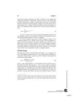
variables is shown in Figure 9.1 for a simple two-dimensional (i.e., two vari-
able) data set. The original data set is shown as a plot of one variable against
the other, a so-called scatter plot, in Figure 9.1A. The variance of variable x
1
is
0.34 and the variance of x
2
is 0.20. After rotation the two new variables, y
1
and
y
2
have variances of 0.53 and 0.005, respectively. This suggests that one vari-
able, y
1
, contains most of the information in the original two-variable set. The
F
IGURE
9.1 A data set consisting of two variables before (left graph) and after
(right graph) linear rotation. The rotated data set still has two variables, but the
variance on one of the variables is quite small compared to the other.
TLFeBOOK
246 Chapter 9

goal of this approach to data reduction is to find a matrix W that will produce
such a transformation.
The two multivariate techniques discussed below, principal component
analysis and independent component analysis, differ in their goals and in the
criteria applied to the transformation. In principal component analysis, the object
is to transform the data set so as to produce a new set of variables (termed
principal components) that are uncorrelated. The goal is to reduce the dimen-
sionality of the data, not necessarily to produce more meaningful variables. We
will see that this can be done simply by rotating the data in M-dimensional
space. In independent component analysis, the goal is a bit more ambitious:
to find new variables (components) that are both statistically independent and
nongaussian.
PRINCIPAL COMPONENT ANALYSIS
Principal component analysis (PCA) is often referred to as a technique for re-
ducing the number of variables in a data set without loss of information, and as
a possible process for identifying new variables with greater meaning. Unfortu-
nately, while PCA can be, and is, used to transform one set of variables into
another smaller set, the newly created variables are not usually easy to interpret.
PCA has been most successful in applications such as image compression where
data reduction—and not interpretation—is of primary importance. In many ap-
plications, PCA is used only to provide information on the true dimensionality
of a data set. That is, if a data set includes M variables, do we really need all
M variables to represent the information, or can the variables be recombined
into a smaller number that still contain most of the essential information (John-
son, 1983)? If so, what is the most appropriate dimension of the new data set?
PCA operates by transforming a set of correlated variables into a new set
of uncorrelated variables that are called the principal components . Note that if
the variables in a data set are already uncorrelated, PCA is of no value. In
addition to being uncorrelated, the principal components are orthogonal and are
ordered in terms of the variability they represent. That is, the first principle

component represents, for a single dimension (i.e., variable ), the greatest amount
of variability in the original data set. Each succeeding orthogonal component
accounts for as much of the remaining variability as possible.
The operation performed by PCA can be described in a number of ways,
but a geometrical interpretation is the most straightforward. While PCA is appli-
cable to data sets containing any number of variables, it is easier to describe
using only two variables since this leads to readily visualized graphs. Figure
9.2A shows two waveforms: a two-variable data set where each variable is a
different mixture of the same two sinusoids added with different scaling factors.
A small amount of noise was also added to each waveform (see Example 9.1).
TLFeBOOK