Biosignal and Biomedical Image Processing MATLAB-Based Applications Muya phần 3 pot

60 Chapter 2
Use a sampling rate of 500 Hz and set the damping factor, δ, to 0.1 and the
frequency, f
n
(termed the undamped natural frequency), to 10 Hz. The array
should be the equivalent of at least 2.0 seconds of data. Plot the impulse re-
sponse to check its shape. Again, convolve this impulse response with a 512-
point noise array and construct and plot the autocorrelation function of this
array. Save the outputs for use in a spectral analysis problem at the end of
Chapter 3. (See Problem 6, Chapter 3.)
8. Construct 4 damped sinusoids similar to the signal, y(t), in Problem 7. Use
a damping factor of 0.04 and generate two seconds of data assuming a sampling
frequency of 500 Hz. Two of the 4 signals should have an f
n
of 10 Hz and the
other two an f
n
of 20 Hz. The two signals at the same frequency should be 90
degrees out of phase (replace the
sin
with a
cos
). Are any of these four signals
orthogonal?
TLFeBOOK
3
Spectral Analysis: Classical Methods
INTRODUCTION
Sometimes the frequency content of the waveform provides more useful infor-
mation than the time domain representation. Many biological signals demon-
strate interesting or diagnostically useful properties when viewed in the so-

called frequency domain. Examples of such signals include heart rate, EMG,
EEG, ECG, eye movements and other motor responses, acoustic heart sounds,
and stomach and intestinal sounds. In fact, just about all biosignals have, at one
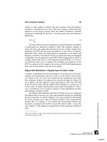
time or another, been examined in the frequency domain. Figure 3.1 shows the
time response of an EEG signal and an estimate of spectral content using the
classical Fourier transform method described later. Several peaks in the fre-
quency plot can be seen indicating significant energy in the EEG at these
frequencies.
Determining the frequency content of a waveform is termed spectral anal-
ysis, and the development of useful approaches for this frequency decomposition
has a long and rich history (Marple, 1987). Spectral analysis can be thought of
as a mathematical prism (Hubbard, 1998), decomposing a waveform into its
constituent frequencies just as a prism decomposes light into its constituent
colors (i.e., specific frequencies of the electromagnetic spectrum).
A great variety of techniques exist to perform spectral analysis, each hav-
ing different strengths and weaknesses. Basically, the methods can be divided
into two broad categories: classical methods based on the Fourier transform and
modern methods such as those based on the estimation of model parameters.
61
TLFeBOOK
62 Chapter 3
F
IGURE
3.1 Upper plot: Segment of an EEG signal from the PhysioNet data bank
(Golberger et al.), and the resultant power spectrum (lower plot).
The accurate determination of the waveform’s spectrum requires that the signal
be periodic, or of finite length, and noise-free. The problem is that in many
biological applications the waveform of interest is either infinite or of sufficient
length that only a portion of it is available for analysis. Moreover, biosignals
are often corrupted by substantial amounts of noise or artifact. If only a portion

of the actual signal can be analyzed, and/or if the waveform contains noise
along with the signal, then all spectral analysis techniques must necessarily be
approximate; they are estimates of the true spectrum. The various spectral analy-
sis approaches attempt to improve the estimation accuracy of specific spectral
features.
Intelligent application of spectral analysis techniques requires an under-
standing of what spectral features are likely to be of interest and which methods
TLFeBOOK
Spectral Analysis: Classical Methods 63
provide the most accurate determination of those features. Two spectral features
of potential interest are the overall shape of the spectrum, termed the spectral
estimate, and/or local features of the spectrum sometimes referred to as paramet-
ric estimates. For example, signal detection, finding a narrowband signal in
broadband noise, would require a good estimate of local features. Unfortunately,
techniques that provide good spectral estimation are poor local estimators and
vice versa. Figure 3.2A shows the spectral estimate obtained by applying the
traditional Fourier transform to a waveform consisting of a 100 Hz sine wave
buried in white noise. The SNR is minus 14 db; that is, the signal amplitude is
1/5 of the noise. Note that the 100 Hz sin wave is readily identified as a peak
in the spectrum at that frequency. Figure 3.2B shows the spectral estimate ob-
tained by a smoothing process applied to the same signal (the Welch method,
described later in this chapter). In this case, the waveform was divided into 32
F
IGURE
3.2 Spectra obtained from a waveform consisting of a 100 Hz sine wave
and white noise using two different methods. The Fourier transform method was
used to produce the left-hand spectrum and the spike at 100 Hz is clearly seen.
An averaging technique was used to create the spectrum on the right side, and
the 100 Hz component is no longer visible. Note, however, that the averaging
technique produces a better estimate of the white noise spectrum. (The spectrum

of white noise should be flat.)
TLFeBOOK
64 Chapter 3
segments, the Fourier transform was applied to each segment, then the 32 spec-
tra were averaged. The resulting spectrum provides a more accurate representa-
tion of the overall spectral features (predominantly those of the white noise),
but the 100 Hz signal is lost. Figure 3.2 shows that the smoothing approach is
a good spectral estimator in the sense that it provides a better estimate of the
dominant noise component, but it is not a good signal detector.
The classical procedures for spectral estimation are described in this chap-
ter with particular regard to their strengths and weaknesses. These methods can
be easily implemented in MATLAB as described in the following section. Mod-
ern methods for spectral estimation are covered in Chapter 5.
THE FOURIER TRANSFORM: FOURIER SERIES ANALYSIS
Periodic Functions
Of the many techniques currently in vogue for spectral estimation, the classical
Fourier transform (FT) method is the most straightforward. The Fourier trans-
form approach takes advantage of the fact that sinusoids contain energy at only
one frequency. If a waveform can be broken down into a series of sines or co-
sines of d iffer ent fr equen cies, the amplitude of these s inusoids must be p ropor -
tional to the frequency component contained in the waveform at those frequencies.
From Fourier series analysis, we know that any periodic waveform can be
represented by a series of sinusoids that are at the same frequency as, or multi-
ples of, the waveform frequency. This family of sinusoids can be expressed
either as sines and cosines, each of appropriate amplitude, or as a single sine
wave of appropriate amplitude and phase angle. Consider the case where sines
and cosines are used to represent the frequency components: to find the appro-
priate amplitude of these components it is only necessary to correlate (i.e., mul-
tiply) the waveform with the sine and cosine family, and average (i.e., integrate)
over the complete waveform (or one period if the waveform is periodic). Ex-

pressed as an equation, this procedure becomes:
a(m) =
1
T
∫
T
0
x(t) cos(2πmf
T
t) dt (1)
b(m) =
1
T
∫
T
0
x(t) sin(2πmf
T
t) dt (2)
where T is the period or time length of the waveform, f
T
= 1/T, and m is set of
integers, possibly infinite: m = 1, 2,3, ,defining the family member. This
gives rise to a family of sines and cosines having harmonically related frequen-
cies, mf
T
.
In terms of the general transform discussed in Chapter 2, the Fourier series
analysis uses a probing function in which the family consists of harmonically
TLFeBOOK

Spectral Analysis: Classical Methods 65
related sinusoids. The sines and cosines in this family have valid frequencies
only at values of m/T, which is either the same frequency as the waveform
(when m = 1) or higher multiples (when m > 1) that are termed harmonics.
Since this approach represents waveforms by harmonically related sinusoids,
the approach is sometimes referred to as harmonic decomposition. For periodic
functions, the Fourier transform and Fourier series constitute a bilateral trans-
form: the Fourier transform can be applied to a waveform to get the sinusoidal
components and the Fourier series sine and cosine components can be summed
to reconstruct the original waveform:
x(t) = a(0)/2 +
∑
∞
m=0
a(k) cos(2πmf
T
t) +
∑
∞
m=0
b(k) sin (2πmf
T
t) (3)
Note that for most real waveforms, the number of sine and cosine compo-
nents that have significant amplitudes is limited, so that a finite, sometimes
fairly short, summation can be quite accurate. Figure 3.3 shows the construction
F
IGURE
3.3 Two periodic functions and their approximations constructed from a
limited series of sinusoids. Upper graphs: A square wave is approximated by a

series of 3 and 6 sine waves. Lower graphs: A triangle wave is approximated by
a series of 3 and 6 cosine waves.
TLFeBOOK
66 Chapter 3
of a square wave (upper graphs) and a triangle wave (lower graphs) using Eq.
(3) and a series consisting of only 3 (left side) or 6 (right side) sine waves. The
reconstructions are fairly accurate even when using only 3 sine waves, particu-
larly for the triangular wave.
Spectral information is usually presented as a frequency plot, a plot of
sine and cosine amplitude vs. component number, or the equivalent frequency.
To convert from component number, m, to frequency, f, note that f = m/T, where
T is the period of the fundamental. (In digitized signals, the sampling frequency
can also be used to determine the spectral frequency). Rather than plot sine and
cosine amplitudes, it is more intuitive to plot the amplitude and phase angle of
a sinusoidal wave using the rectangular-to-polar transformation:
a cos(x) + b sin(x) = C sin(x +Θ) (4)
where C = (a
2
+ b
2
)
1/2
and Θ=tan
−1
(b/a).
Figure 3.4 shows a periodic triangle wave (sometimes referred to as a
sawtooth), and the resultant frequency plot of the magnitude of the first 10
components. Note that the magnitude of the sinusoidal component becomes
quite small after the first 2 components. This explains why the triangle function
can be so accurately represented by only 3 sine waves, as shown in Figure 3.3.

F
IGURE
3.4 A triangle or sawtooth wave (left) and the first 10 terms of its Fourier
series (right). Note that the terms become quite small after the second term.
TLFeBOOK
Spectral Analysis: Classical Methods 67
Symmetry
Some waveforms are symmetrical or anti-symmetrical about t = 0, so that one
or the other of the components, a(k)orb(k) in Eq. (3), will be zero. Specifically,
if the waveform has mirror symmetry about t = 0, that is, x(t) = x(−t), than mul-
tiplications by a sine functions will be zero irrespective of the frequency, and
this will cause all b(k) terms to be zeros. Such mirror symmetry functions are
termed even functions. Similarly, if the function has anti-symmetry, x(t) =−x(t),
a so-called odd function, then all multiplications with cosines of any frequency
will be zero, causing all a(k) coefficients to be zero. Finally, functions that have
half-wave symmetry will have no even coefficients, and both a(k) and b(k) will
be zero for even m. These are functions where the second half of the period
looks like the first half flipped left to right; i.e., x(t) = x(T − t). Functions having
half-wave symmetry can also be either odd or even functions. These symmetries
are useful for reducing the complexity of solving for the coefficients when such
computations are done manually. Even when the Fourier transform is done on
a computer (which is usually the case), these properties can be used to check
the correctness of a program’s output. Table 3.1 summarizes these properties.
Discrete Time Fourier Analysis
The discrete-time Fourier series analysis is an extension of the continuous analy-
sis procedure described above, but modified by two operations: sampling and
windowing. The influence of sampling on the frequency spectra has been cov-
ered in Chapter 2. Briefly, the sampling process makes the spectra repetitive at
frequencies mf
T

(m = 1,2,3, ), and symmetrically reflected about these fre-
quencies (see Figure 2.9). Hence the discrete Fourier series of any waveform is
theoretically infinite, but since it is periodic and symmetric about f
s
/2, all of the
information is contained in the frequency range of 0 to f
s
/2 ( f
s
/2 is the Nyquist
frequency). This follows from the sampling theorem and the fact that the origi-
nal analog waveform must be bandlimited so that its highest frequency, f
MAX
,
is <f
s
/2 if the digitized data is to be an accurate representation of the analog
waveform.
T
ABLE
3.1 Function Symmetries
Function Name Symmetry Coefficient Values
Even x(t) = x(−t) b(k) = 0
Odd x(t) =−x(−t) a(k) = 0
Half-wave x(t) = x(T−t) a(k) = b(k) = 0; for m even
TLFeBOOK
68 Chapter 3
The digitized waveform must necessarily be truncated at least to the length
of the memory storage array, a process described as windowing. The windowing
process can be thought of as multiplying the data by some window shape (see

Figure 2.4). If the waveform is simply truncated and no further shaping is per-
formed on the resultant digitized waveform (as is often the case), then the win-
dow shape is rectangular by default. Other shapes can be imposed on the data
by multiplying the digitized waveform by the desired shape. The influence of
such windowing processes is described in a separate section below.
The equations for computing Fourier series analysis of digitized data are
the same as for continuous data except the integration is replaced by summation.
Usually these equations are presented using complex variables notation so that
both the sine and cosine terms can be represented by a single exponential term
using Euler’s identity:
e
jx
= cos x + j sin x (5)
(Note mathematicians use i to represent
√
−1 while engineers use j; i is reserved
for current.) Using complex notation, the equation for the discrete Fourier trans-
form becomes:
X(m) =
∑
N−1
n=0
x(n)e
(−j2πmn/N )
(6)
where N is the total number of points and m indicates the family member, i.e.,
the harmonic number. This number must now be allowed to be both positive
and negative when used in complex notation: m =−N/2, ,N /2–1. Note the
similarity of Eq. (6) with Eq. (8) of Chapter 2, the general transform in discrete
form. In Eq. (6), f

m
(n) is replaced by e
−j2πmn/N
. The inverse Fourier transform can
be calculated as:
x(n) =
1
N
∑
N−1
n=0
X(m) e
−j2πnf
m
T
s
(7)
Applying the rectangular-to-polar transformation described in Eq. (4), it
is also apparent *X(m)* gives the magnitude for the sinusoidal representation of
the Fourier series while the angle of X(m) gives the phase angle for this repre-
sentation, since X(m) can also be written as:
X(m) =
∑
N−1
n=0
x(n) cos(2πmn/N) − j
∑
N−1
n=0
x(n) sin(2πmn/N) (8)

As mentioned above, for computational reasons, X(m) must be allowed to
have both positive and negative values for m; negative values imply negative
frequencies, but these are only a computational necessity and have no physical
meaning. In some versions of the Fourier series equations shown above, Eq. (6)
TLFeBOOK
Spectral Analysis: Classical Methods 69
is multiplied by T
s
(the sampling time) while Eq. (7) is divided by T
s
so that the
sampling interval is incorporated explicitly into the Fourier series coefficients.
Other methods of scaling these equations can be found in the literature.
The discrete Fourier transform produces a function of m. To convert this
to frequency note that:
f
m
= mf
1
= m/T
P
= m/NT
s
= mf
s
/N (9)
where f
1
≡ f
T

is the fundamental frequency, T
s
is the sample interval; f
s
is the
sample frequency; N is the number of points in the waveform; and T
P
= NTs is
the period of the waveform. Substituting m = f
m
T
s
into Eq. (6), the equation for
the discrete Fourier transform (Eq. (6)) can also be written as:
X(f ) =
∑
N−1
n=0
x(n) e
(−j2πnf
m
T
s
)
(10)
which may be more useful in manual calculations.
If the waveform of interest is truly periodic, then the approach described
above produces an accurate spectrum of the waveform. In this case, such analy-
sis should properly be termed Fourier series analysis, but is usually termed
Fourier transform analysis. This latter term more appropriately applies to aperi-

odic or truncated waveforms. The algorithms used in all cases are the same, so
the term Fourier transform is commonly applied to all spectral analyses based
on decomposing a waveform into sinusoids.
Originally, the Fourier transform or Fourier series analysis was imple-
mented by direct application of the above equations, usually using the complex
formulation. Currently, the Fourier transform is implemented by a more compu-
tationally efficient algorithm, the fast Fourier transform (FFT), that cuts the
number of computations from N
2
to 2 log N, where N is the length of the digital
data.
Aperiodic Functions
If the function is not periodic, it can still be accurately decomposed into sinu-
soids if it is aperiodic; that is, it exists only for a well-defined period of time,
and that time period is fully represented by the digitized waveform. The only
difference is that, theoretically, the sinusoidal components can exist at all fre-
quencies, not just multiple frequencies or harmonics. The analysis procedure is
the same as for a periodic function, except that the frequencies obtained are
really only samples along a continuous frequency spectrum. Figure 3.5 shows
the frequency spectrum of a periodic triangle wave for three different periods.
Note that as the period gets longer, approaching an aperiodic function, the spec-
tral shape does not change, but the points get closer together. This is reasonable
TLFeBOOK
70 Chapter 3
F
IGURE
3.5 A periodic waveform having three different periods: 2, 2.5, and 8
sec. As the period gets longer, the shape of the frequency spectrum stays the
same but the points get closer together.
since the space between the points is inversely related to the period (m/T ).* In

the limit, as the period becomes infinite and the function becomes truly aperi-
odic, the points become infinitely close and the curve becomes continuous. The
analysis of waveforms that are not periodic and that cannot be completely repre-
sented by the digitized data is described below.
*The trick of adding zeros to a waveform to make it appear to a have a longer period (and, therefore,
more points in the frequency spectrum) is another example of zero padding.
TLFeBOOK
Spectral Analysis: Classical Methods 71
Frequency Resolution
From the discrete Fourier series equation above (Eq. (6)), the number of points
produced by the operation is N, the number of points in the data set. However,
since the spectrum produced is symmetrical about the midpoint, N/2 (or f
s
/2 in
frequency), only half the points contain unique information.* If the sampling
time is T
s
, then each point in the spectra represents a frequency increment of
1/(NT
s
). As a rough approximation, the frequency resolution of the spectra will
be the same as the frequency spacing, 1/(NT
s
). In the next section we show that
frequency resolution is also influenced by the type of windowing that is applied
to the data.
As shown in Figure 3.5, frequency spacing of the spectrum produced by
the Fourier transform can be decreased by increasing the length of the data, N.
Increasing the sample interval, T
s

, should also improve the frequency resolution,
but since that means a decrease in f
s
, the maximum frequency in the spectra,
f
s
/2 is reduced limiting the spectral range. One simple way of increasing N even
after the waveform has been sampled is to use zero padding, as was done in
Figure 3.5. Zero padding is legitimate because the undigitized portion of the
waveform is always assumed to be zero (whether true or not). Under this as-
sumption, zero padding simply adds more of the unsampled waveform. The
zero-padded waveform appears to have improved resolution because the fre-
quency interval is smaller. In fact, zero padding does not enhance the underlying
resolution of the transform since the number of points that actually provide
information remains the same; however, zero padding does provide an interpo-
lated transform with a smoother appearance. In addition, it may remove ambigu-
ities encountered in practice when a narrowband signal has a center frequency
that lies between the 1/NT
s
frequency evaluation points (compare the upper two
spectra in Figure 3.5). Finally, zero padding, by providing interpolation, can
make it easier to estimate the frequency of peaks in the spectra.
Truncated Fourier Analysis: Data Windowing
More often, a waveform is neither periodic or aperiodic, but a segment of a
much longer—possibly infinite—time series. Biomedical engineering examples
are found in EEG and ECG analysis where the waveforms being analyzed con-
tinue over the lifetime of the subject. Obviously, only a portion of such wave-
forms can be represented in the finite memory of the computer, and some atten-
tion must be paid to how the waveform is truncated. Often a segment is simply
*Recall that the Fourier transform contains magnitude and phase information. There are N/2 unique

magnitude data points and N/2 unique phase data points, so the same number of actual data points
is required to fully represent the data. Both magnitude and phase data are required to reconstruct
the original time function, but we are often only interested in magnitude data for analysis.
TLFeBOOK
72 Chapter 3
cut out from the overall waveform; that is, a portion of the waveform is trun-
cated and stored, without modification, in the computer. This is equivalent to the
application of a rectangular window to the overall waveform, and the analysis is
restricted to the windowed portion of the waveform. The window function for a
rectangular window is simply 1.0 over the length of the window, and 0.0 else-
where, (Figure 3.6, left side). Windowing has some similarities to the sampling
process described previously and has well-defined consequences on the resultant
frequency spectrum. Window shapes other than rectangular are possible simply
by multiplying the waveform by the desired shape (sometimes these shapes are
referred to as tapering functions). Again, points outside the window are assumed
to be zero even if it is not true.
When a data set is windowed, which is essential if the data set is larger
than the memory storage, then the frequency characteristics of the window be-
come part of the spectral result. In this regard, all windows produce artifact. An
idea of the artifact produced by a given window can be obtained by taking the
Fourier transform of the window itself. Figure 3.6 shows a rectangular window
on the left side and its spectrum on the right. Again, the absence of a window
function is, by default, a rectangular window. The rectangular window, and in
fact all windows, produces two types of artifact. The actual spectrum is widened
by an artifact termed the mainlobe, and additional peaks are generated termed
F
IGURE
3.6 The time function of a rectangular window (left) and its frequency
characteristics (right).
TLFeBOOK

Spectral Analysis: Classical Methods 73
the sidelobes. Most alternatives to the rectangular window reduce the sidelobes
(they decay away more quickly than those of Fig ure 3.6), but at the cost of w id er
mainlobes. Figures 3.7 and 3.8 show the shape and frequency spectra produced
by two popular windows: the triangular window and the raised cosine or Ham-
ming window. The algorithms for these windows are straightforward:
Triangular window:
for odd n:
w(k) =
ͭ
2k/(n − 1)
2(n − k − 1)/(n + 1)
1 ≤ k ≤ (n + 1)/2
(n + 1)/2 ≤ k ≤ n
(11)
for even n:
w(k) =
ͭ
(2k − 1)/n
2(n − k + 1)/n
1 ≤ k ≤ n/2
(n/2) + 1 ≤ k ≤ n
(12)
Hamming window:
w(k + 1) = 0.54 − 0.46(2πk/(n − 1))k = 0,1, ,n − 1 (13)
F
IGURE
3.7 The triangular window in the time domain (left) and its spectral char-
acteristic (right). The sidelobes diminish faster than those of the rectangular win-
dow (Figure 3.6), but the mainlobe is wider.

TLFeBOOK
74 Chapter 3
F
IGURE
3.8 The Hamming window in the time domain (left) and its spectral char-
acteristic (right).
These and seve ra l others are eas il y impl emented in MATLAB, espe cia ll y
with the Signa l Proc es sin g Toolbo x as descr ibed in the next section. A MATLA B
routine is also described to plot the spectral characteristics of these and other
windows. Selecting the appropriate window, like so many other aspects of signal
analysis, depends on what spectral features are of interest. If the task is to
resolve two narrowband signals closely spaced in frequency, then a window
with the narrowest mainlobe (the rectangular window) is preferred. If there is a
strong and a weak signal spaced a moderate distance apart, then a window with
rapidly decaying sidelobes is preferred to prevent the sidelobes of the strong
signal from overpowering the weak signal. If there are two moderate strength
signals, one close and the other more distant from a weak signal, then a compro-
mise window with a moderately narrow mainlobe and a moderate decay in side-
lobes could be the best choice. Often the most appropriate window is selected
by trial and error.
Power Spectrum
The power spectrum is commonly defined as the Fourier transform of the auto-
correlation function. In continuous and discrete notation, the power spectrum
equation becomes:
TLFeBOOK
Spectral Analysis: Classical Methods 75
PS(f ) =
∫
T
0

r
xx
(τ) e
−2πf
T
τ
dτ
PS(f ) =
∑
N−1
n=0
r
xx
(n) e
−j2πnf
T
T
s
(14)
where r
xx
(n) is the autocorrelation function described in Chapter 2. Since the
autocorrelation function has odd symmetry, the sine terms, b(k) will all be zero
(see Table 3.1) and Eq. (14) can be simplified to include only real cosine terms.
PS(f ) =
∫
T
0
r
xx

(τ) cos(2πmf
T
t) dτ
PS(f) =
∑
N−1
n=0
r
xx
(n) cos(2πnf
T
T
s
) (15)
These equations in continuous and discrete form are sometimes referred
to as the cosine transform. This approach to evaluating the power spectrum has
lost favor to the so-called direct approach, given by Eq. (18) below, primarily
because of the efficiency of the fast Fourier transform. However, a variation of
this approach is used in certain time–frequency methods described in Chapter
6. One of the problems compares the power spectrum obtained using the direct
approach of Eq. (18) with the traditional method represented by Eq. (14 ).
The direct approach is motivated by the fact that the energy contained in
an analog signal, x(t), is related to the magnitude of the signal squared, inte-
grated over time:
E =
∫
∞
−∞
*x(t)*
2

dt (16)
By an extension of Parseval’s theorem it is easy to show that:
∫
∞
−∞
*x(t)*
2
dt =
∫
∞
−∞
*X(f )*
2
df (17)
Hence *X( f )*
2
equals the energy density function over frequency, also re-
ferred to as the energy spectral density, the power spectral density, or simply
the power spectrum. In the direct approach, the power spectrum is calculated as
the magnitude squared of the Fourier transform of the waveform of interest:
PS(f ) = *X(f)*
2
(18)
Power spectral analysis is commonly applied to truncated data, particu-
larly when the data contains some noise, since phase information is less useful
in such situations.
TLFeBOOK
76 Chapter 3
While the power spectrum can be evaluated by applying the FFT to the
entire waveform, averaging is often used, particularly when the available wave-

form is only a sample of a longer signal. In such very common situations, power
spectrum evaluation is necessarily an estimation process, and averaging im-
proves the statistical properties of the result. When the power spectrum is based
on a direct application of the Fourier transf orm followed by averagi ng, it is com-
monly referred to as an average periodogram. As with the Fourier transform,
evaluation of power spectra involves necessary trade-offs to produce statistically
reliable spectral estimates that also have high resolution. These trade-offs are
implemented through the selection of the data window and the averaging strat-
egy. In practice, the selection of data window and averaging strategy is usually
based on experimentation with the actual data.
Considerations regarding data windowing have already been described and
apply similarly to power spectral analysis. Averaging is usually achieved by
dividing the waveform into a number of segments, possibly overlapping, and
evaluating the Fourier transform on each of these segments (Figure 3.9). The
final spectrum is taken from an average of the Fourier transforms obtained from
the various segments. Segmentation necessarily reduces the number of data sam-
F
IGURE
3.9 A waveform is divided into three segments with a 50% overlap be-
tween each segment. In the Welch method of spectral analysis, the Fourier trans-
form of each segment would be computed separately, and an average of the
three transforms would provide the output.
TLFeBOOK
Spectral Analysis: Classical Methods 77
ples evaluated by the Fourier transform in each segment. As mentioned above,
frequency resolution of a spectrum is approximately equal to 1/NT
s
, where N is
now the number samples per segment. Choosing a short segment length (a small
N) will provide more segments for averaging and improve the reliability of the

spectral estimate, but it will also decrease frequency resolution. Figure 3.2
shows spectra obtained from a 1024-point data array consisting of a 100 Hz
sinusoid and white noise. In Figure 3.2A, the periodogram is taken from the
entire waveform, while in Figure 3.2B the waveform is divided into 32 non-
overlapping segments; a Fourier transform is calculated from each segment, then
averaged. The periodogram produced from the segmented and averaged data is
much smoother, but the loss in frequency resolution is apparent as the 100 Hz
sine wave is no longer visible.
One of the most popular procedures to evaluate the average periodogram
is attributed to Welch and is a modification of the segmentation scheme origi-
nally developed by Bartlett. In this approach, overlapping segments are used,
and a window is applied to each segment. By overlapping segments, more seg-
ments can be averaged for a given segment and data length. Averaged periodo-
grams obtained from noisy data traditionally average spectra from half-overlap-
ping segments; that is, se gm ent s that overlap by 50%. Hi gh er amount s of overlap
have been recommended in other applications, and, when computing time is
not factor, maximum overlap has been recommended. Maximum overlap means
shifting over by just a single sample to get the new segment. Examples of this
approach are provided in the next section on implementation.
The use of data windowing for sidelobe control is not as important when
the spectra are expected to be relatively flat. In fact, some studies claim that
data windows give some data samples more importance than others and serve
only to decrease frequency resolution without a significant reduction in estima-
tion error. While these claims may be true for periodograms produced using all
the data (i.e., no averaging), they are not true for the Welch periodograms be-
cause overlapping segments serves to equalize data treatment and the increased
number of segments decreases estimation errors. In addition, windows should
be applied whenever the spectra are expected have large amplitude differences.
MATLAB IMPLEMENTATION
Direct FFT and Windowing

MATLAB provides a variety of methods for calculating spectra, particularly if
the Signal Processing Toolbox is available. The basic Fourier transform routine
is implemented as:
X = fft(x,n)
TLFeBOOK
78 Chapter 3
where
X
is the input waveform and
x
is a complex vector providing the sinusoi-
dal coefficients. The argument
n
is optional and is used to modify the length of
data analyzed: if
n < length(x)
, then the analysis is performed over the first
n
points; or, if
n > length(x), x
is padded with trailing zeros to equal
n
. The
fft
routine implements Eq. (6 ) above and employs a high -speed algorithm.
Calculation time is highly dependent on data length and is fastest if the data
length is a power of two, or if the length has many prime factors. For example,
on one machine a 4096-point FFT takes 2.1 seconds, but requires 7 seconds if
the sequence is 4095 points long, and 58 seconds if the sequence is for 4097
points. If at all possible, it is best to stick with data lengths that are powers of

two.
The magnitude of the frequency spectra can be easily obtained by apply-
ing the absolute value function,
abs
, to the complex output
X
:
Magnitude = abs(X)
This MATLAB function simply takes the square root of the sum of the real part
of
X
squared and the imaginary part of
X
squared. The phase angle of the spectra
can be obtained by application of the MATLAB
angle
function:
Phase = angle(X)
The
angle
function takes the arctangent of the imaginary part divided by
the real part of
Y
. The magnitude and phase of the spectrum can then be plotted
using standard MATLAB plotting routines. An example applying the MATLAB
fft
to a array containing sinusoids and white noise is provided below and the
resultant spectra is given in Figure 3.10. Other applications are explored in the
problem set at the end of this chapter. This example uses a special routine,
sig_noise,

found on the disk. The routine generates data consisting of sinu-
soids and noise that are useful in evaluating spectral analysis algorithms. The
calling structure for
sig_noise
is:
[x,t] = sig_noise([f],[SNR],N);
where
f
specifies the frequency of the sinusoid(s) in Hz,
SNR
specifies the de-
sired noise associated with the sinusoid(s) in db, and
N
is the number of points.
The routine assumes a sample frequency of 1 kHz. If
f
and
SNR
are vectors,
multiple sinusoids are generated. The output waveform is in
x
and
t
is a time
vector useful in plotting.
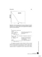
Example 3.1 Plot the power spectrum of a waveform consisting of a
single sine wave and white noise with an SNR of −7 db.
TLFeBOOK
Spectral Analysis: Classical Methods 79
F

IGURE
3.10 Plot produced by the MATLAB program above. The peak at 250
Hz is apparent. The sampling frequency of this data is 1 kHz, hence the spectrum
is symmetric about the Nyquist frequency, f
s
/2 (500 Hz). Normally only the first
half of this spectrum would be plotted (SNR =−7 db; N = 1024).
% Example 3.1 and Figure 3.10 Determine the power spectrum
% of a noisy waveform
% First generates a waveform consisting of a single sine in
% noise, then calculates the power spectrum from the FFT
% and plots
clear all; close all;
N = 1024; % Number of data points
% Generate data using sig_noise
% 250 Hz sin plus white noise; N data points ; SNR = -7 db
[x,t] = sig_noise (250,-7,N);
fs = 1000; % The sample frequency of data
% is 1 kHz.
Y = fft(x); % Calculate FFT
PS = abs(Y).
v
2; % Calculate PS as magnitude
% squared
TLFeBOOK
80 Chapter 3
freq = (1:N)/fs; % Frequency vector for plot-
ting
plot(freq,20*log10(PS),’k’); % Plot PS in log scale
title(’Power Spectrum (note symmetric about fs/2)’);

xlabel(’Frequency (Hz)’);
ylabel(’Power Spectrum (db)’);
The Welch Method for Power Spectral
Density Determination
As described above, the Welch method for evaluating the power spectrum di-
vides the data in several segments, possibly overlapping, performs an FFT on
each segment, computes the magnitude squared (i.e., power spectrum), then
averages these spectra. Coding these in MATLAB is straightforward, but this is
unnecessary as the Signal Processing Toolbox features a function that performs
these operations. In its more general form, the
pwelch
* function is called as:
[PS,f] = pwelch(x,window,noverlap,nfft,fs)
Only the first input argument, the name of the data vector, is required as
the other arguments have default values. By default,
x
is divided into eight
sections with 50% overlap, each section is windowed with a Hamming window
and eight periodograms are computed and averaged. If
window
is an integer, it
specifies the segment length, and a Hamming window of that length is applied
to each segment. If
window
is a vector, then it is assumed to contain the window
function (easily implemented using the window routines described below). In
this situation, the window size will be equal to the length of the vector, usually
set to be the same as
nfft
. If the window length is specified to be less than

nfft
(greater is not allowed), then the window is zero padded to have a length
equal to
nfft
. The argument
noverlap
specifies the overlap in samples. The
sampling frequency is specified by the optional argument
fs
and is used to fill
the frequency vector,
f
, in the output with appropriate values. This output vari-
able can be used in plotting to obtain a correctly scaled frequency axis (see
Example 3.2). As is always the case in MATLAB, any variable can be omitted,
and the default selected by entering an empty vector, [ ].
If
pwelch
is called with no output arguments, the default is to plot the
power spectral estimate in dB per unit frequency in the current figure window.
If
PS
is specified, then it contains the power spectra.
PS
is only half the length
of the data vector,
x
, specifically, either
(nfft/2)؉1
if

nfft
is even, or
(nfft؉1)/2
for
nfft
odd, since the additional points would be redundant. (An
*The calling structure for this function is different in MATLAB versions less than 6.1. Use the
‘Help’ command to determine the calling structure if you are using an older version of MATLAB.
TLFeBOOK
Spectral Analysis: Classical Methods 81
exception is made if
x
is complex data in which case the length of
PS
is equal
to
nfft
.) Other o pt ion s are ava ila bl e and can be found in the help file for
pwelch
.
Example 3.2 Apply Welch’s method to the sine plus noise data used in
Example 3.1. Use 124-point data segments and a 50% overlap.
% Example 3.2 and Figure 3.11
% Apply Welch’s method to sin plus noise data of Figure 3.10
clear all; close all;
N = 1024; % Number of data points
fs = 1000; % Sampling frequency (1 kHz)
F
IGURE
3.11 The application of the Welch power spectral method to data con-

taining a single sine wave plus noise, the same as the one used to produce
the spectrum of Figure 3.10. The segment length was 128 points and segments
overlapped by 50%. A triangular window was applied. The improvement in the
background spectra is obvious, although the 250 Hz peak is now broader.
TLFeBOOK
82 Chapter 3
% Generate data (250 Hz sin plus noise)
[x,t,] = sig_noise(250,-7,N);
%
% Estimate the Welch spectrum using 128 point segments,
% a the triangular filter, and a 50% overlap.
%
[PS,f] = (x, triang(128),[ ],128,fs);
plot(f,PS,’k’); % Plot power spectrum
title(’Power Spectrum (Welch Method)’);
xlabel(’Frequency (Hz)’);
ylabel(’Power Spectrum’);
Comparing the spectra in Figure 3.11 with that of Figure 3.10 shows that
the background noise is considerably smoother and reduced. The sine wave at
250 Hz is clearly seen, but the peak is now slightly broader indicating a loss in
frequency resolution.
Window Functions
MATLAB has a number of data windows available including those de-
scribed in Eqs. (11–13). The relevant MATLAB routine generates an n-point
vector array containing the appropriate window shape. All have the same
form:
w = window_name(N); % Generate vector w of length N
% containing the window function
% of the associated name
where

N
is the number of points in the output vector and
window_name
is the
name, or an abbreviation of the name, of the desired window. At this writing,
thirteen different windows are available in addition to rectangular
(rectwin)
which is included for completeness. Using
help window
will provide a list of
window names. A few of the more popular windows are:
bartlett
,
blackman
,
gausswin
,
hamming
(a common MATLAB default window),
hann
,
kaiser
, and
triang
. A few of the routines have additional optional arguments. In particu-
lar,
chebwin
(Chebyshev window), which features a nondecaying, constant
level of sidelobes, has a second argument to specify the sidelobe amplitude. Of
course, the smaller this level is set, the wider the mainlobe, and the poorer the

frequency resolution. Details for any given window can be found through the
help
command. In addition to the individual functions, all of the window func-
tions can be constructed with one call:
w = window(@name,N,opt) % Get N-point window ‘name.’
TLFeBOOK
Spectral Analysis: Classical Methods 83
where name is the name of the specific window function (preceded by
@
),
N
the
number of points desired, and
opt
possible optional argument(s) required by
some specific windows.
To apply a window to the Fourier series analysis such as in Example
2.1, simply point-by-point multiply the digitized waveform by the output of the
MATLAB
window_name
routine before calling the FFT routine. For example:
w = triang (N); % Get N-point triangular window curve
x = x .* w’; % Multipl y (point-by-point) data by wind ow
X = fft(x); % Calculate FFT
Note that in the example above it was necessary to transpose the window
function
W
so that it was in the same format as the data. The window function
produces a row vector.
Figure 3.12 shows two spectra obtained from a data set consisting of two

sine waves closely spaced in frequency (235 Hz and 250 Hz) with added white
noise in a 256 point array sampled at 1 kHz. Both spectra used the Welch
method with the same parameters except for the windowing. (The window func-
F
IGURE
3.12 Two spectra computed for a waveform consisting of two closely
spaced sine waves (235 and 250 Hz) in noise (SNR =−10 db). Welch’s method
was used for both methods with the same parameters (nfft = 128, overlap = 64)
except for the window functions.
TLFeBOOK
84 Chapter 3
tion can be embedded in the
pwelch
calling structure.) The upper spectrum was
obtained using a Hamming window (
hamming
) which has large sidelobes, but a
fairly narrow mainlobe while the lower spectrum used a Chebyshev window
(
chebwin
) which has small sidelobes but a larger mainlobe.
A small difference is seen in the ability to resolve the two peaks. The
Hamming window with a smaller main lobe gives rise to a spectrum that shows
two peaks while the presence of two peaks might be missed in the Chebyshev
windowed spectrum.
PROBLEMS
1. (A) Construct two arrays of white noise: one 128 points in length and the
other 1024 points in length. Take the FT of both. Does increasing the length
improve the spectral estimate of white noise?
(B) Apply the Welch methods to the longer noise array using a Hanning window

with an nfft of 128 with no overlap. Does this approach improve the spectral
estimate? Now change the overlap to 64 and note any changes in the spectrum.
Submit all frequency plots appropriately labeled.
2. Find the power spectrum of the filtered noise data from Problem 3 in Chap-
ter 2 using the standard FFT. Show frequency plots appropriately labeled. Scale,
or rescale, the frequency axis to adequately show the frequency response of this
filter.
3. Find the power spectrum of the filtered noise data in Problem 2 above using
the FFT, but zero pad the data so that N = 2048. Note the visual improvement
in resolution.
4. Repeat Problem 2 above using the data from Problem 6 in Chapter 2.
Applying the Hamming widow to the data before calculating the FFT.
5. Repeat problem 4 above using the Welch method with 256 and 65 segment
lengths and the window of your choice.
6. Repeat Problem 4 above using the data from Problem 7, Chapter 2.
7. Use routine
sig_noise
noise to generate a 256-point array that contains
two closely spaced sinusoids at 140 and 180 Hz both with an SNR of -10 db.
(Callin g stru ct ure :
data = sig_noise([140 180], [-10 -10], 256);)
Sig_noise
assumes a sampling rate of 1 kHz. Use the Welch method. Find the
spectrum of the waveform for segment lengths of 256 (no overlap) and 64 points
with 0%, 50% and 99% overlap.
8. Use
sig_noise
to generate a 512-point array that contains a single sinusoid
at 200 Hz with an SNR of -12 db. Find the power spectrum first by taking the
TLFeBOOK