GIÁO TRÌNH KHAI THÁC PHẦN mềm TRONG GIA CÔNG KHUÔN mẫu chapter III strain

1
Chapter III: Strain
1
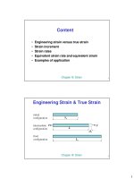
Content
• Engineering strain versus true strain
• Strain increment
• Strain rates
• Equivalent strain rate and equivalent strain
• Examples of application
Chapter III: Strain
2
Engineering Strain & True Strain
λ
λλ
λ
0
λ
λλ
λ
λ
λλ
λ
1
intermediate
configuration
initial
configuration
final
configuration
F
F

d
λ
λλ
λ
2
Chapter III: Strain
3
Mechanical engineering strain:
1 0
0
e
−
=
l l
l
Elongation is based to the initial length.
1
0
1
0
ln
d d
d
ε ε
 
= → = =
 
 
∫
l

l
l l l
l l l
True (logarithmic, natural) strain:
Forming technology is related to the actual length, useful to
describe the large amounts of deformation.
Chapter III: Strain
4
Remark on Plastic Strains
elastic plastic
ε ε ε
= +
The total strain can be splitted (phân tách) into:
In metalforming, plastic strains are much larger than elastic ones:
plastic
ε ε
≈
since
3
Chapter III: Strain
5
Examples
Example 3.1:
a) A uniform bar of length λ
0
is uniformly extended until its final
length is λ = 2 λ
0
. Compute the values of engineering strain and
true strain for this extension.

b) To what final length, λ, must a bar of initial length λ
0
, be
compressed if the strains are to be the same (except for sign) as
those in part (a)?
Example 3.2:
A uniform bar of 100 mm initial length is elongated to a length of 200
mm in three stages:
Stage 1: 100 mm to 120 mm, Stage 2: 120 mm to 150 mm and
Stage 3: 150 mm to 200 mm.
Calculate the engineering and true strains for each stage and
compare the sums of the three with the overall values of the strains.
Chapter III: Strain
6
Engineering Strain & True Strain
( )
01
0 0 0
ln ln ln 1 ln 1
e
ε
     
+ ∆
∆
= = = + = +
     
     
l ll
l
l l l

( )
2 3
ln 1
2 3
e e
e e
ε
= + ≈ − + −
K
Series expansion:
Hence:
0
e e
ε
→ →
e
0.001 0.010 0.02 0.05 0.10 0.20 0.50 1.0
ε
εε
ε
0.0009995 0.00995 0.0198 0.0487 0.0953 0.182 0.405 0.693
ε/
ε/ε/
ε/
e
0.9995 0.995 0.990 0.976 0.953 0.912 0.811 0.693
4
Chapter III: Strain
7
Advantages and disadvantages resulting from the

calculation with e and ɛ
Large strains lead to numerical values which are not easy to deal with.
(True strain ɛ=1 equals percentage strain of about 173%.)
The logarithmic strain is mechanical more sensible as the strain related to
the initial length and present calculation advantages. So in procedures
with several forming steps the total strain equals the summation of the
single strains.
In contrast to (ngược với) the strain the true strain take in consideration
not only the initial and the end state but also all intermediate steps of the
total forming.
In the calculation with strains only, the single strains can not be added to
the total strain, because they are related to the initial length.
Chapter III: Strain
8
Definition: True Strain
The point has initial
coordinations: x, y, z,
After forming it has current
coordinations: x’, y’, z’.
Displacements of point
following x, y, z directions
are:
x’ - x = u
x
= u
y’ - y = u
y
= v
z’ - z = u
z

= w
Elongations and Deformations angle (Shear Strain) on area z
5
Chapter III: Strain
9
True Strain Differentials
Similarly we can define the true strain differentials:
{ }
x
y
z
xy
i yz
zx
yx
zy
xz
d
d
d
d
E E d
d
d
d
d
ε
ε
ε
ε

ε
ε
ε
ε
ε
 
 
 
 
 
 
 
= =
 
 
 
 
 
 
 
 
where:
(
)
, etc.
x
du
d
x
ε

∂
=
∂
(
)
(
)
1
, etc.
2
xy
du dv
d
y x
ε
 ∂ ∂ 
= +
 
∂ ∂
 
Here: u, v and w are displacements in x,
y and z directions and x, y, z are current
coordinates.
Chapter III: Strain
10
True Strain Differentials
T
x xy xz
yx y yz
zx zy z

ε
ε γ γ
γ ε γ
γ γ ε
=
















1
2
1
2
1
2
1
2
1

2
1
2
ε
ε ε ε
ε ε ε
ε ε ε
ij
xx xy xz
yx yy yz
zx zy zz
=










Tensor of strain:
ε
∂
∂
ε
∂
∂
ε

∂
∂
x
x
y
y
z
z
u
x
u
y
u
z
=
=
=











∂
∂

+
∂
∂
=γ
∂
∂
+
∂
∂
=γ
∂
∂
+
∂
∂
=γ
z
u
x
u
y
u
z
u
x
u
y
u
xz
zx

z
y
yz
y
x
xy
Where:
6
Chapter III: Strain
11
Strain Rates
(
)
x
du
d
x
ε
∂
=
∂
Sometimes it is more convenient (thuận tiện) to introduce strain rates:
Consider the strain differential:
Dividing both sides by the differential time dt :
(
)
x
du
d
dt

dt x
ε
∂
=
∂
Or:
(
)
x
x
du dt
d
u
dt x x
ε
ε
∂
∂
= = =
∂ ∂
&
&
Sometimes the strain-rate tensor is called “Rate-of-Deformation”
tensor
ij ij
D
ε
=
&
Chapter III: Strain

12
Strain Rates
(
)
( )
xx
xx
du dt
d
du x u
dt dt x x
ε
ε
∂
∂ ∂ ∂
= = = =
∂ ∂
&
&
(
)
( )
yy
yy
d
dv dt
dv y v
dt dt y y
ε
ε

∂
∂ ∂ ∂
= = = =
∂ ∂
&
&
[ ]
1
( ) ( )
1
2
2
xy
xy yx
dv x du y
d
v u
dt dt x y
ε
ε ε
∂ ∂ + ∂
 
∂ ∂
= = = = +
 
∂ ∂
 
& &
& &
Similar to strain, we have terms of strain rates:

7
Chapter III: Strain
13
Strain Rate Tensor
xx xy xz
ij yx yy yz
zx zy zz
ε ε ε
ε ε ε ε
ε ε ε
 
 
≡
 
 
 
& & &
& & & &
& & &
xx
u
x
ε
∂
=
∂
&
&
yy
v

y
ε
∂
=
∂
&
&
zz
w
z
ε
∂
=
∂
&
&
1
2
xz zx
w u
x z
ε ε
∂ ∂
 
= = +
 
∂ ∂
 
& &
& &

1
2
xy yx
v u
x y
ε ε
 
∂ ∂
= = +
 
∂ ∂
 
& &
& &
1
2
yz zy
v w
z y
ε ε
 
∂ ∂
= = +
 
∂ ∂
 
& &
& &
Normal Strain Rate Components:
Shear Strain Rate

Components:
The Strain Rate Tensor in 3-D:
particle velocity in -direction
particle velocity in -direction
particle velocity in -direction
u x
v y
w z
&
&
&
Chapter III: Strain
14
Examples
Example 2.3:
A uniform bar with current length λ is extended at its free end by a
tool with velocity of v
tool
. Determine the strain rate in axial
direction.
λ
λλ
λ
v
tool
Example 2.4:
A sheet with dimensions shown in
the figure is sheared by a tool
with velocity v
tool

. Determine the
shear strain rate.
v
tool
y
x
h
8
Chapter III: Strain
15
Strain Rates in Cylindrical Coordinate System
z
r
θ
P
(r, ,z)
θ
1 1
2
1 1
2
1
2
r
r r
z
z z
r z
zr rz
u u

u
r r
u u
r z
u u
z r
θ
θ θ θ
θ
θ θ
ε ε
θ
ε ε
θ
ε ε
∂ ∂
 
 
= = − +
 
 
∂ ∂
 
 
∂ ∂
 
= = +
 
∂ ∂
 

∂ ∂
 
= = +
 
∂ ∂
 
& &
& &
&
& &
& &
& &
& &
,
,
1
r
rr r r r
z
zz z z
u u
u u
r r
u
u
z
θ
θθ
ε ε
θ

ε
∂ ∂
 
= = = +
 
∂ ∂
 
∂
= =
∂
& &
& &
& &
&
&
&
rr r rz
ij r z
zr z zz
θ
θ θθ θ
θ
ε ε ε
ε ε ε ε
ε ε ε
 
 
≡
 
 

 
& & &
& & & &
& & &
Chapter III: Strain
16
Strain Rates for Axisymmetrical Problems
Conditions of axial symmetry:
0 and 0 where stands for any quant
ity
u
θ
θ
∂ ⊗
= = ⊗
∂
&
Using these conditions results:
, ,
1
r z
rr r r r zz z z
u u
u u u
r r z
θθ
ε ε ε
∂ ∂
= = = = =
∂ ∂

& &
& & &
& & &
1
0 0
2
r z
r r z z zr rz
u u
z r
θ θ θ θ
ε ε ε ε ε ε
∂ ∂
 
= = = = = = +
 
∂ ∂
 
& &
& & & & & &
9
Chapter III: Strain
17
Strain Rates in Spherical Coordinate System
{ }
( )
,
,
,
r, ,

, ,
, ,
1 1
cot
sin
1

1 1 1

2 sin
1 1
cot
2 sin
1 1

2
rr r r
r
r
r r r
r r r r
u
u u u
r
u u
r
u u u
r
u u u
r

u u u
r
ϕϕ ϕ ϕ θ
θθ θ θ
ϕ ϕ ϕ ϕ ϕ
ϕθ θϕ θ ϕ θ ϕ ϕ
θ θ θ θ θ
ε
ε θ
θ
ε
ε ε
θ
ε ε θ
θ
ε ε
=
 
= + +
 
 
= +
 
 
= = − +
 
 
 
 
 

= = + −
 
 
 
= = + −
 

&
&
&
& & &
&
& &
& &
& & &
& &
& & &
& &
& & &

r
θ
P
(r, )
ϕ,
θ
ϕ
Chapter III: Strain
18
Strain Rates in Spherical Coordinate System:

Symmetry
For symmetry with:
0 and u u
ϕ θ
ϕ
∂ ⊗
= =
∂
& &
,
,
,
0

2
r
rr r r
r r
r
r r
u
u
r
u
r
ϕϕ θθ
ϕ ϕ ϕθ θϕ
θ
θ θ
ε ε ε

ε ε ε ε
ε ε
= = =
= = = =
= =
&
& & &
&
& & & &
&
& &
10
Chapter III: Strain
19
Total Finite Strains
Total finite strains have physical meaning if and only if:
1. All shear strain rates are zero,
2. The straining path is straight,
0
ij
i j
ε
= ∀ ≠
&
constant, etc.
xx yy
ε ε
=
& &
λ

λλ
λ
v
tool
d
x
x
Assuming uniform straining:
tool
x
u v
=
&
l
( )
{
tool
xx
u x
v
u du
x dx
ε
∂
= = =
∂
&
& &
&
l

tool
d
v
dt
=
l
but
so that
xx
d dt
ε
=
l
&
l
Integration:
0
0 0
t t
xx xx
d dt d
dt dt
ε ε
= = = ⇒
∫ ∫ ∫
l
l
l l
&
l l

0
ln
xx
ε
=
l
l
Chapter III: Strain
20
Principal Strains
x
y
z
1
2
3
element before
deformation
element after
deformation
(
)
( )
( )
1 1 0
2 1 0
3 1 0
ln
ln
ln

a a
b b
c c
ε
ε
ε
=
=
=
principal
strain
directions
11
Chapter III: Strain
21
Equivalent Plastic Strain
The hardening of metals in multidimensional strain states
is represented by the equivalent strain and its rate. The
von Mises equivalent plastic strain rate can be derived as:
( ) ( )
2 2 2 2 2 2
2
2
3
xx yy zz xy yz xz
ε ε ε ε ε ε ε
 
= + + + + +
 
&

& & & & & &
The total equivalent strain is simply:
t
dt
ε ε
=
∫
&
In terms of principal strains:
( )
2 2 2
1 2 3
2
3
ε ε ε ε
= + +
Chapter III: Strain
22
Condition of Volume Constancy (1)
During plastic deformations volume of the deformed body
remains constant (experimental observations).
0 0 0 1 1 1
final
initial
V a b c a b c const
= × × = × × =
1424314243
0
dV
dt

∴ =
12
Chapter III: Strain
23
Condition of Volume Constancy (2)
( )
1 1 1
0
dV d
a b c
dt dt
= = ⋅ ⋅
1 1 1
1 1 1 1 1 1 1 1 1
0
da db dc
dV
b c a c a b a b c
dt dt dt dt
     
= = ⋅ ⋅ + ⋅ ⋅ + ⋅ ⋅
     
     
1 1 1
1 1 1
0
da db dc
a dt b dt c dt
= + + ⇒
1 2 3

0
ε ε ε
= + +
& & &
{
!
tensor
⇒
0
xx yy zz
ε ε ε
= + +
& & &
Expand (khai triển)
Chapter III: Strain
24
Examples (1)
Example 2.5:
Consider the frictionless axisym-
metrical upsetting process as
shown in the figure. Determine the
equivalent plastic strain for the
process by assuming that there is
no bulging and the cylinder is
compressed from height h
0
to h
1
.
F, v

tool
u
r
.
r
z
D
h
lower die
(fixed)
upper die
(moving)
13
Chapter III: Strain
25
Equivalent Strain Rate in Upsetting
0
1
2
3
4
0 10 20 30 40 50 60 70
Height Reduction in %
Equivalent Strain Rate in 1/s
v
tool
= 100 mm/s, h
0
= 100 mm
0%

60%
40%
20%
Chapter III: Strain
26
Equivalent Plastic Strain in Upsetting
0
1
2
3
0 20 40 60 80 100
Height Reduction in %
Equivalent Strain
v
tool
= 100 mm/s, h
0
= 100 mm
0%
80%
60%40%
20%
0
/
h h
∆
14
Chapter III: Strain
27
Examples (2)

Example 2.6:
Consider the frictionless
axisymmetrical drawing
process as shown in the
figure. Determine the
equivalent plastic strain
rate for the process by
assuming that the axial
velocity component is a
function of the axial
coordinate only.