flexibility value of distributed generation in transmission expansion planning

Flexibility Value of Distributed Generation in Transmission Expansion Planning 351
Flexibility Value of Distributed Generation in Transmission Expansion
Planning
Paúl Vásquez and Fernando Olsina
X

Flexibility Value of Distributed Generation in
Transmission Expansion Planning

Paúl Vásquez
1
and Fernando Olsina
2
1
Consejo Nacional de Electricidad (CONELEC), Ecuador

2
Institute of Electrical Energy (IEE), CONICET, Argentina

1. Introduction
The efficiency of the classic planning methods for solving realistic problems largely relies on
an accurate prediction of the future. Nevertheless, the presence of strategic uncertainties in
current electricity markets has made prediction and even forecasting essentially futile. The
new paradigm of decision-making involves two major deviations from the conventional
planning approach. On one hand, the acceptation the fact the future is almost unpredictable.
On the other hand, the application of solid risk management techniques turns to be
indispensable.
In this chapter, a decision-making framework that properly handles strategic uncertainties is
proposed and numerically illustrated for solving a realistic transmission expansion planning
problem.
The key concept proposed in this chapter lies in systematically incorporating flexible

options such as large investments postponement and investing in Distributed Generation, in
foresight of possible undesired events that strategic uncertainties might unfold. Until now,
the consideration of such flexible options has remained largely unexplored. The
understanding of the readers is enhanced by means of applying the proposed framework in
a numerical mining firm expansion capacity planning problem. The obtained results show
that the proposed framework is able to find solutions with noticeably lower involved risks
than those resulting from traditional expansion plans.
The remaining of this chapter is organized as follows. Section 2 is devoted to describe the
main features of the transmission expansion problem and the opportunities for
incorporating flexibility in transmission investments for managing long-term planning risks.
The most salient characteristics of the several formulations proposed in the literature for
solving the optimization problem are reviewed and discussed along Section 3. The several
types of uncertain information that must be handled within the optimization problem are
classified and analyzed in Section 4. The proposed framework for solving the stochastic
optimization problem considering the value provided to expansion plans by flexible
investment projects is presented in Section 5. In Section 6, an illustrative-numerical example
based on an actual planning problem illustrates the applicability of the developed flexibility-
based planning approach. Concluding remarks of Section 7 close this chapter.

16
www.intechopen.com
Distributed Generation 352
2. The transmission expansion planning
Since the beginning of the power industry, steadily growing demand for electricity and
generation commonly located distant from consumption centres have led to the need of
planning for adapted transmission networks aiming at transport the electric energy from
production sites towards consumption areas in an efficient manner. In the vertically
integrated power industry, the responsibility for optimally driving the expansion of
transmission networks has typically lied with a centralized planner.
During the last two decades, stimulating competition has been a way to increase the

efficiency of utilities as well as to improve the overall performance of the liberalized
electricity industry (Rudnick & Zolezzi, 2000; Gómez Expósito). Because of the large
economies of scales, a unique transmission company is typically responsible for delivering
the power generation to the load points. Under this paradigm, the transmission activity has
special significance since it allows competition among market participants. In addition, the
transmission infrastructure largely determines the economy and the reliability level that the
power system can achieve. For this reasons, planning for efficient transmission expansions is
a critical activity. With the aim of solving the transmission expansion planning problem
(TEP), a great number of approaches have been devised (Latorre et al., 2003; Lee et al., 2006).
A classic TEP task entails determining ex-ante the location, capacity, and timing of
transmission expansion projects in order to deliver maximal social welfare over the planning
period while maintaining adequate reliability levels (Willis, 1997). Under this traditional
perspective, the TEP problem can be mathematically formulated as a large scale, multi-
period, non-linear, mixed-integer and constrained optimization problem. In practice,
however, such a rigorous formulation is unfeasible to be solved. Planners typically solve the
TEP problem under a very simplified framework, e.g. static (one-stage) formulations, where
timing of decisions is not a decision variable (Latorre et al., 2003).

2.1 The emerging new TEP problem
The improvement of computing technology with increasingly faster processors along with
the option of solving the problem in a distributed computing environment has made
possible to handle a bigger number of parameters and variables and even formulate the TEP
as a multi-period optimization problem (Youssef, 2001; Braga & Saraiva, 2005). However,
jointly with the above mentioned increasing competition brought by the deregulation,
relevant aspects such as: the development of new small-scale generation technologies
(Distributed Generation, DG), the improvement of power electronic devices (e.g. FACTS),
the environmental concerns that makes more difficult to obtain new right-of-way for
transmission lines, the lack of regulatory incentives to investing in transmission projects,
among others, have increased considerably the dynamic of power markets, the number of
variables and parameters to be considered, and the uncertainties involved. Accordingly, the

TEP problem is now substantially more complex (Buygi, 2004; Neimane, 2001).
Under this perspective, ad doc adjustments of expansion plans or additional contingent
investments made in order to mitigate the harmful economic consequences that unexpected
events have demonstrated the limited practical efficiency of applying classic TEP models
(Añó et al., 2005). In fact, the substantial risks involved in planning decisions emphasize the
need of developing practical methodological tools which allow for the assessment and the
risk management.
2.2 Nature of transmission investments
Due to some singular characteristics, transmission investments exhibit a distinctive nature
with respect to other related investment problems (Kirschen & Strbac, 2004; Dixit &
Pindyck, 1994):
Capital intensive: because of the substantial economies of scale, large and infrequent
transmission investments are often preferred, involving huge financial commitments.
One-step investments: a substantial fraction of total capital expenditures must be
committed before the new transmission equipment can be commissioned.
Long recovering times: transmission lines, transformers, etc. are expected to be paid-off
after several years or even decades.
Long-run uncertainties: transmission investments are vulnerable to unanticipated scenarios
that can take place in the long-term future. Future demand, fuel costs, and generation
investments are uncertain variables at the planning stage.
Low adaptability: transmission projects are typically unable to be adapted to circumstances
that considerably differ from the planning conditions. An unadapted transmission system
entails considerable loss of social welfare.
Irreversibility: once incurred, transmission investments are considered sunk costs. Indeed,
it is very unlikely that transmission equipment can serve other purposes if conditions
changes unfavourably. Under these circumstances the transmission equipment could not be
sold off without assuming significant losses on its nominal value.
Postponability: In general, opportunities for investing in transmission equipment are not of
the type “now or never”. Thus, it is valuable to leave the investment option open, i.e. wait
for valuable, arriving information until uncertainties are partially resolved. Thus,

transmission investment projects can be treated in the same way as a financial call option.
The opportunity cost of losing the ability to defer a decision while looking for better
information should be properly considered.
Due to the mentioned features, transmission network expansions traditionally respond to
the demand growth by infrequently investing in large and efficient projects. Consequently,
traditional solutions to the TEP inevitably entail two evident intrinsic weaknesses:

 Because only large projects are economically efficient, planners have a limited number
of alternatives and consequently the solutions found provide low levels of
adaptability to the demand growth, and
 To drive the expansion, enormous irreversible upfront efforts in capital and time are
required.

The huge uncertainties of the problem interact with the irreversible nature of transmission
investments for radically increasing the risk present in expansion decisions. Such interaction
has been ignored in traditional models at the moment of evaluating expansion strategies.
More recently, it has been recognized that conventional decision-making approaches usually
leads to the wrong investment decisions (Dixit & Pindyck, 1994). Therefore, the interaction
between uncertainties and the nature of transmission investments must be properly
accounted for.

www.intechopen.com
Flexibility Value of Distributed Generation in Transmission Expansion Planning 353
2. The transmission expansion planning
Since the beginning of the power industry, steadily growing demand for electricity and
generation commonly located distant from consumption centres have led to the need of
planning for adapted transmission networks aiming at transport the electric energy from
production sites towards consumption areas in an efficient manner. In the vertically
integrated power industry, the responsibility for optimally driving the expansion of
transmission networks has typically lied with a centralized planner.

During the last two decades, stimulating competition has been a way to increase the
efficiency of utilities as well as to improve the overall performance of the liberalized
electricity industry (Rudnick & Zolezzi, 2000; Gómez Expósito). Because of the large
economies of scales, a unique transmission company is typically responsible for delivering
the power generation to the load points. Under this paradigm, the transmission activity has
special significance since it allows competition among market participants. In addition, the
transmission infrastructure largely determines the economy and the reliability level that the
power system can achieve. For this reasons, planning for efficient transmission expansions is
a critical activity. With the aim of solving the transmission expansion planning problem
(TEP), a great number of approaches have been devised (Latorre et al., 2003; Lee et al., 2006).
A classic TEP task entails determining ex-ante the location, capacity, and timing of
transmission expansion projects in order to deliver maximal social welfare over the planning
period while maintaining adequate reliability levels (Willis, 1997). Under this traditional
perspective, the TEP problem can be mathematically formulated as a large scale, multi-
period, non-linear, mixed-integer and constrained optimization problem. In practice,
however, such a rigorous formulation is unfeasible to be solved. Planners typically solve the
TEP problem under a very simplified framework, e.g. static (one-stage) formulations, where
timing of decisions is not a decision variable (Latorre et al., 2003).

2.1 The emerging new TEP problem
The improvement of computing technology with increasingly faster processors along with
the option of solving the problem in a distributed computing environment has made
possible to handle a bigger number of parameters and variables and even formulate the TEP
as a multi-period optimization problem (Youssef, 2001; Braga & Saraiva, 2005). However,
jointly with the above mentioned increasing competition brought by the deregulation,
relevant aspects such as: the development of new small-scale generation technologies
(Distributed Generation, DG), the improvement of power electronic devices (e.g. FACTS),
the environmental concerns that makes more difficult to obtain new right-of-way for
transmission lines, the lack of regulatory incentives to investing in transmission projects,
among others, have increased considerably the dynamic of power markets, the number of

variables and parameters to be considered, and the uncertainties involved. Accordingly, the
TEP problem is now substantially more complex (Buygi, 2004; Neimane, 2001).
Under this perspective, ad doc adjustments of expansion plans or additional contingent
investments made in order to mitigate the harmful economic consequences that unexpected
events have demonstrated the limited practical efficiency of applying classic TEP models
(Añó et al., 2005). In fact, the substantial risks involved in planning decisions emphasize the
need of developing practical methodological tools which allow for the assessment and the
risk management.
2.2 Nature of transmission investments
Due to some singular characteristics, transmission investments exhibit a distinctive nature
with respect to other related investment problems (Kirschen & Strbac, 2004; Dixit &
Pindyck, 1994):
Capital intensive: because of the substantial economies of scale, large and infrequent
transmission investments are often preferred, involving huge financial commitments.
One-step investments: a substantial fraction of total capital expenditures must be
committed before the new transmission equipment can be commissioned.
Long recovering times: transmission lines, transformers, etc. are expected to be paid-off
after several years or even decades.
Long-run uncertainties: transmission investments are vulnerable to unanticipated scenarios
that can take place in the long-term future. Future demand, fuel costs, and generation
investments are uncertain variables at the planning stage.
Low adaptability: transmission projects are typically unable to be adapted to circumstances
that considerably differ from the planning conditions. An unadapted transmission system
entails considerable loss of social welfare.
Irreversibility: once incurred, transmission investments are considered sunk costs. Indeed,
it is very unlikely that transmission equipment can serve other purposes if conditions
changes unfavourably. Under these circumstances the transmission equipment could not be
sold off without assuming significant losses on its nominal value.
Postponability: In general, opportunities for investing in transmission equipment are not of
the type “now or never”. Thus, it is valuable to leave the investment option open, i.e. wait

for valuable, arriving information until uncertainties are partially resolved. Thus,
transmission investment projects can be treated in the same way as a financial call option.
The opportunity cost of losing the ability to defer a decision while looking for better
information should be properly considered.
Due to the mentioned features, transmission network expansions traditionally respond to
the demand growth by infrequently investing in large and efficient projects. Consequently,
traditional solutions to the TEP inevitably entail two evident intrinsic weaknesses:

 Because only large projects are economically efficient, planners have a limited number
of alternatives and consequently the solutions found provide low levels of
adaptability to the demand growth, and
 To drive the expansion, enormous irreversible upfront efforts in capital and time are
required.

The huge uncertainties of the problem interact with the irreversible nature of transmission
investments for radically increasing the risk present in expansion decisions. Such interaction
has been ignored in traditional models at the moment of evaluating expansion strategies.
More recently, it has been recognized that conventional decision-making approaches usually
leads to the wrong investment decisions (Dixit & Pindyck, 1994). Therefore, the interaction
between uncertainties and the nature of transmission investments must be properly
accounted for.

www.intechopen.com
Distributed Generation 354
2.3 New available flexible options
Although the major negative concerns regarding classic TEP models have been analyzed, in
this work potential positive aspects are also considered and exploited. In fact, available
technical and managerial embedded options exhibit some desirable features such as: modularity,
scalability, short lead times, high levels of reversibility, and smaller financial commitments.
This option can be incorporated as novel decision choices that a planner has available for

reducing the planning risks as well as for improving the quality of the found solutions.
In this sense, planners must rely on an expansion model able to capture all major
complexities present in the TEP in order to properly manage the involved huge long-term
uncertainties and deal with the problem of dimensionality.
The key underlying assumption of conventional probabilistic models is the passive
planner’s attitude regarding future unexpected circumstances. In fact, available choices for
reacting to the several scenarios which could take place overtime are ignored during the
planning process. However, in practice planners have the ability to adapt their investment
strategies in response to undesired or unanticipated events.
Hence, planning for contingent scenarios by exploiting technical and managerial options
embedded in transmission investment projects is a effective mean for satisfactorily dealing
with the current TEP problem

2.4 The flexibility value of Distributed Generation
Distributed Generation is defined as a source of electric energy located very close to the
demand (Ackerman et al., 2001; Pepermans et al., 2003). Usually, DG investments are neither
more efficient nor more economic than conventional generation or transmission expansions,
which still enjoy of significant economies of scale such. Nevertheless, important
contributions of DG occur when: energy T&D costs are avoided, demand uses it for peak
shaving, losses are reduced, network reliability is increased, or when it lead to investment
deferral in T&D systems (Jenkins et al., 2000; Willis & Scott, 2000; Brown et al., 2001; Grijalva
& Visnesky, 2005).
DG seems a plausible means of improving the traditional way of driving the expansion of
the transmission systems. Delaying investments in T&D systems by investing in DG is one
of the major motivations and research topics of this work (Brown et al., 2001; Daly &
Morrison, 2001; Vignolo & Zeballos, 2001; Dale, 2002; Vásquez & Olsina, 2007).
The fact of considering DG projects as new decision alternatives within the TEP, involves
the incorporation of additional parameters such as investment and production costs of DG
technologies, firm power, etc.
Based on the typical short lead times of DG projects and their lower irreversibility, the

uncertainty present in DG project investment decisions and investment costs can be
neglected. Provided that the DG technologies considered in this work are fuel-fired plants,
the availability of the DG could be modelled by assessing only availability factors (Samper
& Vargas, 2006).

3. State-of-art of the TEP optimization approaches
The successful development of an efficient and practical expansion model primarily
depends on considering the following topics: the planner’s objectives, the availability and
quality of the information to be handled as well as the depth level at which the planner
decides to face the problem. In this sense, a set of basic elements that the planner must
consider and specify before mathematically formulating the problem are summarized in the
Table 1.

Topic Concern Recommended Value Symbol
Scales



of time
Planning horizon 10 to 15 years
T
Decision periods ≥ 1 year
p
Sub-periods
resolution
Weekly, monthly, seasonally

subp
Demand duration
curve

Peak, valley, mid-load P(t), Q(t)
Decision
alternatives
Alternatives that
planner has
available for drivin
g
the expansion
Expansion strategy S
k
, S
f

Large transmission projects D
k
(p)
Defer transmission projects
O
k
(p)
Invest in DG projects
Type of alternative [0,1,2,3 n]
Investment decision timing
p
Decision alternative location

( )
f
bus

Objective
function (C
k
)
components
Efficiency in
investments,
operative efficienc
y
,
reliability and
technical feasibility

Investment costs
C
I
, C
IDG

Operative costs C
G
,C
GDG

O&M costs C
O&M

VOLL or EENS costs C
LOL

Active power losses costs -
Constraints
Transmission
expansion plans
performance
assessment subject
to:
Power balance S
G
+ S
D
= S
L

Voltage limits V
j min
, V
j max

Generators capacity limits P
i min
, P
i max

DG plants capacity limits
DG
i min
, DG
i
max

Transmission lines power
flow limits
F
l

Budgetary constraints -
Input
parameters
Certain Certain S(t)
Uncertain
Random
X(t)
Truly uncertain
Fuzzy -
Table 1. Basic elements to be defined before devising a TEP methodology

The current TEP problem can be described as the constant planners’ dilemma of deciding on
a sequential combination of large transmission projects and new available flexible options,
which allows the planners to efficiently adapting their decisions to unexpected
circumstances that may take place during the planning period.
Under this novel paradigm, TEP is a multi-period decision-making problem which entails
determining ex-ante the right type, location, capacity, and timing of a set of available
decision options in order to deliver a maximal expected social welfare as well as suitably
reducing the existing risks over the planning period.
Probabilistic decision theory, i.e. the probabilistic choice paradigm, is well-known and has
been extensively applied in several stochastic optimization problems. However, a
probabilistic decision formulation within the TEP is an intractable task and its application
www.intechopen.com
Flexibility Value of Distributed Generation in Transmission Expansion Planning 355

2.3 New available flexible options
Although the major negative concerns regarding classic TEP models have been analyzed, in
this work potential positive aspects are also considered and exploited. In fact, available
technical and managerial embedded options exhibit some desirable features such as: modularity,
scalability, short lead times, high levels of reversibility, and smaller financial commitments.
This option can be incorporated as novel decision choices that a planner has available for
reducing the planning risks as well as for improving the quality of the found solutions.
In this sense, planners must rely on an expansion model able to capture all major
complexities present in the TEP in order to properly manage the involved huge long-term
uncertainties and deal with the problem of dimensionality.
The key underlying assumption of conventional probabilistic models is the passive
planner’s attitude regarding future unexpected circumstances. In fact, available choices for
reacting to the several scenarios which could take place overtime are ignored during the
planning process. However, in practice planners have the ability to adapt their investment
strategies in response to undesired or unanticipated events.
Hence, planning for contingent scenarios by exploiting technical and managerial options
embedded in transmission investment projects is a effective mean for satisfactorily dealing
with the current TEP problem

2.4 The flexibility value of Distributed Generation
Distributed Generation is defined as a source of electric energy located very close to the
demand (Ackerman et al., 2001; Pepermans et al., 2003). Usually, DG investments are neither
more efficient nor more economic than conventional generation or transmission expansions,
which still enjoy of significant economies of scale such. Nevertheless, important
contributions of DG occur when: energy T&D costs are avoided, demand uses it for peak
shaving, losses are reduced, network reliability is increased, or when it lead to investment
deferral in T&D systems (Jenkins et al., 2000; Willis & Scott, 2000; Brown et al., 2001; Grijalva
& Visnesky, 2005).
DG seems a plausible means of improving the traditional way of driving the expansion of
the transmission systems. Delaying investments in T&D systems by investing in DG is one

of the major motivations and research topics of this work (Brown et al., 2001; Daly &
Morrison, 2001; Vignolo & Zeballos, 2001; Dale, 2002; Vásquez & Olsina, 2007).
The fact of considering DG projects as new decision alternatives within the TEP, involves
the incorporation of additional parameters such as investment and production costs of DG
technologies, firm power, etc.
Based on the typical short lead times of DG projects and their lower irreversibility, the
uncertainty present in DG project investment decisions and investment costs can be
neglected. Provided that the DG technologies considered in this work are fuel-fired plants,
the availability of the DG could be modelled by assessing only availability factors (Samper
& Vargas, 2006).

3. State-of-art of the TEP optimization approaches
The successful development of an efficient and practical expansion model primarily
depends on considering the following topics: the planner’s objectives, the availability and
quality of the information to be handled as well as the depth level at which the planner
decides to face the problem. In this sense, a set of basic elements that the planner must
consider and specify before mathematically formulating the problem are summarized in the
Table 1.

Topic Concern Recommended Value Symbol
Scales



of time
Planning horizon 10 to 15 years
T
Decision periods ≥ 1 year
p
Sub-periods

resolution
Weekly, monthly, seasonally

subp
Demand duration
curve
Peak, valley, mid-load P(t), Q(t)
Decision
alternatives
Alternatives that
planner has
available for drivin
g
the expansion
Expansion strategy S
k
, S
f

Large transmission projects D
k
(p)
Defer transmission projects
O
k
(p)
Invest in DG projects
Type of alternative [0,1,2,3 n]
Investment decision timing
p

Decision alternative location

( )
f
bus

Objective
function (C
k
)
components
Efficiency in
investments,
operative efficiency,
reliability and
technical feasibility

Investment costs
C
I
, C
IDG

Operative costs C
G
,C
GDG

O&M costs C
O&M

VOLL or EENS costs C
LOL

Active power losses costs -
Constraints
Transmission
expansion plans
performance
assessment subject
to:
Power balance S
G
+ S
D
= S
L

Voltage limits V
j min
, V
j max

Generators capacity limits P
i min
, P
i max

DG plants capacity limits
DG

i min
, DG
i
max

Transmission lines power
flow limits
F
l

Budgetary constraints -
Input
parameters
Certain Certain S(t)
Uncertain
Random
X(t)
Truly uncertain
Fuzzy -
Table 1. Basic elements to be defined before devising a TEP methodology

The current TEP problem can be described as the constant planners’ dilemma of deciding on
a sequential combination of large transmission projects and new available flexible options,
which allows the planners to efficiently adapting their decisions to unexpected
circumstances that may take place during the planning period.
Under this novel paradigm, TEP is a multi-period decision-making problem which entails
determining ex-ante the right type, location, capacity, and timing of a set of available
decision options in order to deliver a maximal expected social welfare as well as suitably
reducing the existing risks over the planning period.
Probabilistic decision theory, i.e. the probabilistic choice paradigm, is well-known and has

been extensively applied in several stochastic optimization problems. However, a
probabilistic decision formulation within the TEP is an intractable task and its application
www.intechopen.com
Distributed Generation 356
has only been feasible when very strong simplifications are adopted by planners (Neimane,
2001). This work proposes a practical framework for treating the TEP. Even though a
number of simplifications are still necessary, the main features of the new TEP problem are
retained.
The analysis of the state-of-art of the TEP solutions approaches sets as a start point the
classic stochastic optimization problem formulation. Under the assumption of inelastic
demand behaviour, the optimization problem can be rigorously stated as follows:

{ }
( ) ( )
0
E[ ]
f f
opt opt
i
T
S
S S S S
opt OF opt OF C dF C
Î Î
W
ì ü
ï ï
ï ï
ï ï
ï ï

=
í ý
ï ï
ï ï
ï ï
ï ï
î þ
ò ò ò

(1)
where, the performance measure of the optimization is the expected present value of the
objective function E[OF(C)] evaluated over a planning horizon T, for a proposed expansion
strategy S.
f
S
is the set of all feasible states of the network, F(C) is the distribution function
of the expansion costs function
1 2 3 i
C(C ,C ,C , ,C ) . The planning period T usually only can
take discrete values
0 1 2 3
p
t ,t ,t ,t , ,t
, and Ω is the domain of existence of C(X,S). The
expansion costs function depends on several uncertain input parameters
( )
1 2 3 n
X x (t),x (t),x (t), ,x (t)
which change over the time, as well as depending on the state of
the network, which also varies over the time

(
)
1 2 3 d
S s (t),s (t),s (t), ,s (t)
. It is important to
note that the problem is subject to a set of constraints, namely Kirchhoff's laws, upper and
lower generation plants capacity limits, transmission lines capacity limits, upper and lower
voltage and phase nodes limits, and budgetary constraints, among others, which are
represented by means of equality and inequality equations. With these considerations, (1)
can be rewritten as follows:

{ }
(
)
( ) ( )
. 1
E[ ] ,
f f
opt opt
n p
S S S S
opt OF opt OF C X S d X
Î
+
Î
Y
ì ü
ï ï
ï ï
ï ï

ï ï
é ù
= F
í ý
ë û
ï ï
ï ï
ï ï
ï ï
î þ
ò ò

(2)
subject to:
( ) ( ) ( )
( )
( )
( )
1min 1 2 max
1min 2 2 max
min max
, , ,
,
,

,
A B L
m m m
P X S P X S P X S
b g X S b

b g X S b
b g X S b
+ =
£ £
£ £
£ £
  

where
( )
F X
is the
( )
1n p+ -dimensional function of probability distributions of input
parameters and
Y
is the domain of existence of the input parameters X.
Formulating
(
)
XF , which incorporates the information about the uncertainties that largely
influence the solution, is a complex task as it involves determining probabilities and
distribution functions of
( )
+1n p

uncertain parameters. However, the more difficult (and in
some cases impossible) task is the formulation of the objective function OF(C). In this sense
the most common simplification considered by TEP models is
( ) ( )

, ,OF C X S C X S
é
ù
=
ë
û
and (2)
can be rewritten as:

{ }
( )
( ) ( )
. 1
min E[ ] min ,
f f
opt opt
n p
S
S S S S
C C X S d X
Î
+
Î
Y
ì ü
ï ï
ï ï
ï ï
ï ï
= F

í ý
ï ï
ï ï
ï ï
ï ï
î þ
ò ò

(3)
which implies that the objective function can be entirely described by the expansion costs
function. In this case the planning problem is often reduced to the minimization of the
expected total expansion costs. Although the complexity of the problem is greatly reduced,
such a formulation does not take into account desires of the decision-maker for reducing
risks present in the expansion decisions. Eventually, this risk neutral formulation may lead
to wrong decisions.
On the other hand, considerable difficulties are related to the computational effort necessary
for efficiently assess the multidimensional integral and for proposing the corresponding
optimization procedure. The only method for dealing with (3) as strict as possible, given
that the
( )
+1n p -dimensional integral must be solved, is applying Monte-Carlo simulation
techniques for evaluating the attributes of the objective function.
There are
( )
(
)
+ +n d
p
1
input parameters in the expansion costs function

1,0 n,0 n,p 1,0 d,p
C(x , x , ,x , s , s )
, from which
( )
1d p +
are decision variables. Assuming as I
the number of available decision choices in each possible right-of-way d, the number of
possible candidate solutions are
(
)
1d p
I
+
. Additionally, by denoting as N the number of
simulations that requires the Monte Carlo simulation, the number of simulations to be
performed depends on the number of periods of time as
( )
1N p + . It is important to
mention that N depends on the degree of confidence that the planner demands on the
results. Under these considerations, the number of required computations for rigorously
evaluating the multidimensional integral and therefore for finding the global optimum is
( )
( )
1
1
d p
N p I
+
+
. Unfortunately performing this task in a real multi-period TEP is not

possible since the number of simulations dramatically increases with the result of
multiplying the possible links and the time periods
( )
1d p + . Due to this fact, researchers
have proposed diverse approaches in order to make the TEP feasible and, in some cases, to
incorporate the desires of the decision-maker for reducing the planning risks. According to
the reviewed literature such simplifications can be categorized as static, deterministic and
non-deterministic formulations of the TEP.

3.1 Static formulation
When the planner demands on further simplifying a deterministic formulation, the
intertemporal dependences and the dynamic nature of the TEP problem is not considered.
Such a formulation is named static. This is a deterministic formulation that entails finding
the optimal state of the network for a future fixed year. Consequently, the input parameters
X do not change during the whole solving process. In this case, there are
+n d
input
parameters within the expansion costs function
21 n 1 d
C(x ,x , ,x , s , s )
from which
d
are
www.intechopen.com
Flexibility Value of Distributed Generation in Transmission Expansion Planning 357
has only been feasible when very strong simplifications are adopted by planners (Neimane,
2001). This work proposes a practical framework for treating the TEP. Even though a
number of simplifications are still necessary, the main features of the new TEP problem are
retained.
The analysis of the state-of-art of the TEP solutions approaches sets as a start point the

classic stochastic optimization problem formulation. Under the assumption of inelastic
demand behaviour, the optimization problem can be rigorously stated as follows:

{ }
( ) ( )
0
E[ ]
f f
opt opt
i
T
S
S S S S
opt OF opt OF C dF C
Î Î
W
ì ü
ï ï
ï ï
ï ï
ï ï
=
í ý
ï ï
ï ï
ï ï
ï ï
î þ
ò ò ò


(1)
where, the performance measure of the optimization is the expected present value of the
objective function E[OF(C)] evaluated over a planning horizon T, for a proposed expansion
strategy S.
f
S
is the set of all feasible states of the network, F(C) is the distribution function
of the expansion costs function
1 2 3 i
C(C ,C ,C , ,C ) . The planning period T usually only can
take discrete values
0 1 2 3
p
t ,t ,t ,t , ,t
, and Ω is the domain of existence of C(X,S). The
expansion costs function depends on several uncertain input parameters
( )
1 2 3 n
X x (t),x (t),x (t), ,x (t)
which change over the time, as well as depending on the state of
the network, which also varies over the time
( )
1 2 3 d
S s (t),s (t),s (t), ,s (t)
. It is important to
note that the problem is subject to a set of constraints, namely Kirchhoff's laws, upper and
lower generation plants capacity limits, transmission lines capacity limits, upper and lower
voltage and phase nodes limits, and budgetary constraints, among others, which are
represented by means of equality and inequality equations. With these considerations, (1)
can be rewritten as follows:

{ }
( )
( ) ( )
. 1
E[ ] ,
f f
opt opt
n p
S S S S
opt OF opt OF C X S d X
Î
+
Î
Y
ì ü
ï ï
ï ï
ï ï
ï ï
é ù
= F
í ý
ë û
ï ï
ï ï
ï ï
ï ï
î þ
ò ò


(2)
subject to:
( ) ( ) ( )
( )
( )
( )
1min 1 2 max
1min 2 2 max
min max
, , ,
,
,

,
A B L
m m m
P X S P X S P X S
b g X S b
b g X S b
b g X S b
+ =
£ £
£ £
£ £
  

where
( )
F X

is the
( )
1n p+ -dimensional function of probability distributions of input
parameters and
Y
is the domain of existence of the input parameters X.
Formulating
( )
XF , which incorporates the information about the uncertainties that largely
influence the solution, is a complex task as it involves determining probabilities and
distribution functions of
( )
+1n p

uncertain parameters. However, the more difficult (and in
some cases impossible) task is the formulation of the objective function OF(C). In this sense
the most common simplification considered by TEP models is
(
)
( )
, ,OF C X S C X S
é ù
=
ë û
and (2)
can be rewritten as:

{ }
( )
( ) ( )

. 1
min E[ ] min ,
f f
opt opt
n p
S
S S S S
C C X S d X
Î
+
Î
Y
ì ü
ï ï
ï ï
ï ï
ï ï
= F
í ý
ï ï
ï ï
ï ï
ï ï
î þ
ò ò

(3)
which implies that the objective function can be entirely described by the expansion costs
function. In this case the planning problem is often reduced to the minimization of the
expected total expansion costs. Although the complexity of the problem is greatly reduced,

such a formulation does not take into account desires of the decision-maker for reducing
risks present in the expansion decisions. Eventually, this risk neutral formulation may lead
to wrong decisions.
On the other hand, considerable difficulties are related to the computational effort necessary
for efficiently assess the multidimensional integral and for proposing the corresponding
optimization procedure. The only method for dealing with (3) as strict as possible, given
that the
( )
+1n p -dimensional integral must be solved, is applying Monte-Carlo simulation
techniques for evaluating the attributes of the objective function.
There are
( )
(
)
+ +n d
p
1
input parameters in the expansion costs function
1,0 n,0 n,p 1,0 d,p
C(x , x , ,x , s , s )
, from which
( )
1d p +
are decision variables. Assuming as I
the number of available decision choices in each possible right-of-way d, the number of
possible candidate solutions are
( )
1d p
I
+

. Additionally, by denoting as N the number of
simulations that requires the Monte Carlo simulation, the number of simulations to be
performed depends on the number of periods of time as
( )
1N p + . It is important to
mention that N depends on the degree of confidence that the planner demands on the
results. Under these considerations, the number of required computations for rigorously
evaluating the multidimensional integral and therefore for finding the global optimum is
(
)
(
)
1
1
d p
N p I
+
+
. Unfortunately performing this task in a real multi-period TEP is not
possible since the number of simulations dramatically increases with the result of
multiplying the possible links and the time periods
( )
1d p + . Due to this fact, researchers
have proposed diverse approaches in order to make the TEP feasible and, in some cases, to
incorporate the desires of the decision-maker for reducing the planning risks. According to
the reviewed literature such simplifications can be categorized as static, deterministic and
non-deterministic formulations of the TEP.

3.1 Static formulation
When the planner demands on further simplifying a deterministic formulation, the

intertemporal dependences and the dynamic nature of the TEP problem is not considered.
Such a formulation is named static. This is a deterministic formulation that entails finding
the optimal state of the network for a future fixed year. Consequently, the input parameters
X do not change during the whole solving process. In this case, there are
+n d
input
parameters within the expansion costs function
21 n 1 d
C(x ,x , ,x , s , s )
from which
d
are
www.intechopen.com
Distributed Generation 358
decision variables. Assuming as I the number of available decision choices in each possible
right-of-way d, the number of possible solutions is
d
I . For instance, in a small TEP problem
with d = 11 and five decision choices on each right-of-way I = 5, the number of possible
combinations is
11 7
5 4.88 10= ⋅ .

3.2 Deterministic formulation
Deterministic models are nowadays widely used in practice for transmission network
planning. This type of models assumes that all the input parameters and variables are
known with complete certainty and, therefore, there is a unique and known scenario for the
evolution of all input parameters. Consequently, there is no need to use probability
distribution functions and the complexity of the optimization process is greatly reduced.
Thus, deterministic formulation entails finding the optimal state of the network over a

planning horizon T, given that the evolution of X along the time is known with certainty.
There are
( )
( )
+ +n d p 1 input parameters inside the expansion costs function
1,0 n,0 n,p 1,0 d,p
C(x , x , ,x , s , s )
from which
( )
1d p + are decision variables. Assuming as I
the number of available decision choices in each possible right-of-way d, the number of
possible solutions to be evaluated for finding the global optimum is
(
)
1d p
I
+
. For instance, in
a small TEP problem with eleven possible new right-of-ways d = 11, five decision choices in
each right-of-way I = 5, and only two decision periods p+1 = 2, the number of possible
combinations are
( )
11. 1 1 15
5 2.38 10
+
= ⋅
.
In this work, the subject of optimization is the present value of the total expansion costs
function C(X,S), evaluated along a planning horizon T, for a proposed expansion strategy S.
C(X,S) is a non-linear function subject to a set of constraints, i.e. Kirchhoff's laws, generation

plants capacity limits and transfer capacity of transmission lines, among others. Such
constraints are represented by means of equality and inequality equations.


{ }
(
)
{
}
min min ,
f f
opt opt
S
S S S S
C C X S
Î Î
=
(4)

( )
( )
( )
( )
( )
( )
( )
( )
( )
&
0

, , , ,
,
1 1 1 1
T
I Gen O M LoL
t t t t
t
C X S C X S C X S C X S
C X S
r r r r
=
é ù
ê ú
= + + +
ê ú
ê ú
+ + + +
ë û
å
(5)
( ) ( ) ( ) ( )
( )
( )
( )
1min 1 2max
1min 2 2max
min max
subject to:
, , , ,
,

,

,
A B R L
m m m
P X S P X S P X S P X S
b g X S b
b g X S b
b g X S b
+ + + =
£ £
£ £
£ £
  

where
( , ) :
I
C X S
Investment costs of the new expansion decisions.
( , ) :
Gen
C X S
Production costs of the different generations units.
&
( , ):
O M
C X S
Annual O&M costs of the transmission network elements.
( , ) :

LoL
C X S
Loss of load annual costs.
:r
Annual discount rate.

3.3 Non-deterministic formulation
Basically non-deterministic formulations of the TEP problem are able to consider the
possible events which could take place in the future by taking into account the uncertainty
present in the information. In this category, the TEP problem can be solved either by means
of a stochastic optimization-based formulation, where the objective function is typically
formulated in term of an expected value or by means of a decision-making framework,
which encompasses a deterministic optimization plus a decision tree analysis. Unfolding
uncertainties are incorporated as branches and decisions are made on the evaluation of the
consequences of deciding on the different expansion alternatives. In this sense, the decision-
making framework allows the planners to gain insight into the risks involved in each
expansion choice and could even suggest new and improved alternatives.
The dimension of the search space for the different TEP formulations depends on the
number of decision choices, the number of decision variables and the number of periods.
Additionally, the degree of detail of the model describing the temporal evolution of the PES
along the planning horizon, namely demand discretization, time resolution and extent of the
planning horizon is another important aspect to take into account since the computational
effort for evaluating each combination depends on it.
To reasonably accomplish the challenging task of solving the TEP problem from a non-
deterministic perspective, require incorporating and modeling a variety of data of diverse
nature. Moreover, due to the large problem size, which is clearly defined by its stochastic,
multi-period, multi-criteria and combinatorial nature, substantial efforts are required in
order to sustain the viability of the proposed models. In this sense, an adequate treatment of
the different types of the information is one of the most important stages before formulating
the non-deterministic TEP model.

4. Handling information within the TEP

The process of solving actual planning problems requires handling a large amount of
information from which only a small fraction is known with complete certainty. In this
section, the major uncertainties affecting the TEP and referred to as variables that affect the
outcomes of decisions and which are not known at time of planning, are analyzed and
categorized from a descriptive viewpoint. Excluded here are the uncertainties originated in
the model’s user, i.e. what is not captured by the model but desired by the user, as well as
uncertainties originated in the model (i.e. the “right” model structure, modelling techniques
and tools).

4.1 Uncertainties present in the TEP
Data about the current state of the network is much more accurate than forecasted data.
Furthermore, uncertainties present in forecasted data are very diverse in nature (Neimane,
www.intechopen.com
Flexibility Value of Distributed Generation in Transmission Expansion Planning 359
decision variables. Assuming as I the number of available decision choices in each possible
right-of-way d, the number of possible solutions is
d
I . For instance, in a small TEP problem
with d = 11 and five decision choices on each right-of-way I = 5, the number of possible
combinations is
11 7
5 4.88 10= ⋅ .

3.2 Deterministic formulation
Deterministic models are nowadays widely used in practice for transmission network
planning. This type of models assumes that all the input parameters and variables are
known with complete certainty and, therefore, there is a unique and known scenario for the

evolution of all input parameters. Consequently, there is no need to use probability
distribution functions and the complexity of the optimization process is greatly reduced.
Thus, deterministic formulation entails finding the optimal state of the network over a
planning horizon T, given that the evolution of X along the time is known with certainty.
There are
( )
(
)
+ +n d p 1 input parameters inside the expansion costs function
1,0 n,0 n,p 1,0 d,p
C(x , x , ,x , s , s )
from which
( )
1d p + are decision variables. Assuming as I
the number of available decision choices in each possible right-of-way d, the number of
possible solutions to be evaluated for finding the global optimum is
(
)
1d p
I
+
. For instance, in
a small TEP problem with eleven possible new right-of-ways d = 11, five decision choices in
each right-of-way I = 5, and only two decision periods p+1 = 2, the number of possible
combinations are
( )
11. 1 1 15
5 2.38 10
+
= ⋅

.
In this work, the subject of optimization is the present value of the total expansion costs
function C(X,S), evaluated along a planning horizon T, for a proposed expansion strategy S.
C(X,S) is a non-linear function subject to a set of constraints, i.e. Kirchhoff's laws, generation
plants capacity limits and transfer capacity of transmission lines, among others. Such
constraints are represented by means of equality and inequality equations.


{ }
(
)
{ }
min min ,
f f
opt opt
S
S S S S
C C X S
Î Î
=
(4)

( )
( )
( )
( )
( )
( )
( )
( )

( )
&
0
, , , ,
,
1 1 1 1
T
I Gen O M LoL
t t t t
t
C X S C X S C X S C X S
C X S
r r r r
=
é
ù
ê
ú
= + + +
ê
ú
ê
ú
+ + + +
ë
û
å
(5)
( ) ( ) ( ) ( )
( )

( )
( )
1min 1 2max
1min 2 2max
min max
subject to:
, , , ,
,
,

,
A B R L
m m m
P X S P X S P X S P X S
b g X S b
b g X S b
b g X S b
+ + + =
£ £
£ £
£ £
  

where
( , ) :
I
C X S
Investment costs of the new expansion decisions.
( , ) :
Gen

C X S
Production costs of the different generations units.
&
( , ):
O M
C X S
Annual O&M costs of the transmission network elements.
( , ) :
LoL
C X S
Loss of load annual costs.
:r
Annual discount rate.

3.3 Non-deterministic formulation
Basically non-deterministic formulations of the TEP problem are able to consider the
possible events which could take place in the future by taking into account the uncertainty
present in the information. In this category, the TEP problem can be solved either by means
of a stochastic optimization-based formulation, where the objective function is typically
formulated in term of an expected value or by means of a decision-making framework,
which encompasses a deterministic optimization plus a decision tree analysis. Unfolding
uncertainties are incorporated as branches and decisions are made on the evaluation of the
consequences of deciding on the different expansion alternatives. In this sense, the decision-
making framework allows the planners to gain insight into the risks involved in each
expansion choice and could even suggest new and improved alternatives.
The dimension of the search space for the different TEP formulations depends on the
number of decision choices, the number of decision variables and the number of periods.
Additionally, the degree of detail of the model describing the temporal evolution of the PES
along the planning horizon, namely demand discretization, time resolution and extent of the
planning horizon is another important aspect to take into account since the computational

effort for evaluating each combination depends on it.
To reasonably accomplish the challenging task of solving the TEP problem from a non-
deterministic perspective, require incorporating and modeling a variety of data of diverse
nature. Moreover, due to the large problem size, which is clearly defined by its stochastic,
multi-period, multi-criteria and combinatorial nature, substantial efforts are required in
order to sustain the viability of the proposed models. In this sense, an adequate treatment of
the different types of the information is one of the most important stages before formulating
the non-deterministic TEP model.

4. Handling information within the TEP

The process of solving actual planning problems requires handling a large amount of
information from which only a small fraction is known with complete certainty. In this
section, the major uncertainties affecting the TEP and referred to as variables that affect the
outcomes of decisions and which are not known at time of planning, are analyzed and
categorized from a descriptive viewpoint. Excluded here are the uncertainties originated in
the model’s user, i.e. what is not captured by the model but desired by the user, as well as
uncertainties originated in the model (i.e. the “right” model structure, modelling techniques
and tools).

4.1 Uncertainties present in the TEP
Data about the current state of the network is much more accurate than forecasted data.
Furthermore, uncertainties present in forecasted data are very diverse in nature (Neimane,
www.intechopen.com
Distributed Generation 360
2001). Therefore, it is recognized the importance of categorizing the uncertain information to
be incorporated within TEP models.
In this work, it is assumed that forecasts and characterization of the forecast uncertainty are
provided to the planning activity. Instead, the attention of this research work is posed in
categorizing all the information to be handled within the TEP and proposing a systematic

methodology for properly incorporating uncertain information of various source and nature
within the TEP model.

4.2 Certain Information
Certain data are those parameters which can be defined explicitly (Neimane, 2001). This
category includes the present network configuration, electrical parameters of the network
components, possible expansion choices and their electrical parameters capacity limits of
transmission lines, nominal voltages and voltage limits.

4.3 Information subjetc to stochastic uncertainty
Uncertainty in data mostly appears due to the inevitable errors incurred when forecasts are
performed. When it is possible to objectively assess the magnitude of such errors with a
satisfactory degree of confidence, then the uncertainty is said to be of random nature (Buygi,
2004). The uncertainty of such variables can be adequately represented by means of
probability distribution functions. Demand, fuel prices and hydrologic resources evolution
are typical examples belonging to this category. In (Vásquez et al., 2008) a well-founded
means for modelling random uncertainties is extensively presented.

4.4 Uncertain non-random information
When it is not possible to estimate with a satisfactory degree of confidence the errors
incurred when forecasts are performed, information is deemed to be of a non-random
nature (Buygi, 2004). Uncertainties in this group are related to human processes (e.g.
investors decisions, changes in regulation, planners and managers investment strategies,
beliefs or subjective judgments). In fact, the future does not appear to be predictable through
extrapolation of historical trends applied to the current environment (Clemons & Barnett,
2003). Thus, non-random uncertainties assessment is derived from decision-makers
perception, experience, expertise and reasoning. Inside this group there are two types of
uncertainties.
The first type belongs to a large amount of valuable information that only can be expressed
in linguistic form, e.g. “satisfactory”, “considerable”, “large”, “small”, “efficient”, etc.

Although this
vague information has a very subjective nature and usually is based on
expert judgment, it can be useful during the decision-making process. Fuzzy sets theory is a
well-founded approach for modelling properly these kinds of uncertainties (Buygi, 2004).
The second type of non-random uncertain information is distinguished by holding
uncertainties typical of dynamic environments that undergo severe and unexpected
changes. This is the case with the TEP environment. According to the literature, these kinds
of uncertainties are known as
strategic uncertainties (Clemons & Barnett, 2003; Brañas et al.,
2004; Detre et al., 2006). A specific feature of them is that they are gradually solved as new
information arrives over time and, once enough information is known, the uncertainty is
solved and disappears definitively (Dillon & Haimes, 1996; Clemons & Barnett, 2003).
Within the TEP problem, this uncertainty affects crucial events that could take place in the
future, such as the generation expansion evolution or the delay on the expansion projects
completion. Data with strategic uncertainties are considered the most important information
to be handled within TEP since they are fundamental drivers of PES evolution and,
therefore, of this decision-making problem. For further reading about this topic see (Detre et
al., 2006). On the other hand, within the PES planning environment, there are not much
bibliographic references about modelling of strategic uncertainties in planning models. In
(Neimane, 2001), this type of information has been designated as truly uncertain
information
1
. Either discrete probability distribution functions or a scenarios technique are
proposed for modelling information of this kind.
Taking into account the above mentioned, in this work it is proposed to model truly
uncertain information by means of discrete probability distribution functions (PDF) where
the probabilities assigned to the occurrence of different scenarios are assumed as known
information. In this sense, a reasonable way for dealing with these two types of uncertainties
is proposed in (Vásquez et al., 2008).

5. The proposed flexibility-based TEP framework
The described TEP problem can be suitably faced by applying the decision tree technique,
which basically consists in decomposing the whole problem into a number w of less
complex sub-problems, each one concerned with solving a multi-period deterministic
optimization as well as assessing the attributes of the expansion plans.
A sub-problem or complete path is represented by a number P of sequential discrete events.
Such events are specified by the assumed discrete nature of strategic uncertainties. Under
these conditions, each sub-problem handles only random uncertainties. Therefore, the
different feasible expansion plans can be valued by applying a probabilistic analysis of the
attributes of the objective function and decisions are made by applying a robustness-based
risk management technique.
A master dynamic programming (DP) problem, by means of a backward induction of P
sequential decisions, makes it possible to incorporate flexible options and, subsequently,
rank the new flexible expansion strategies.
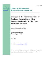
The entire proposed methodology, can be described as follows in five stages and illustrated
in Fig. 1:

1.
To decompose the TEP problem into w sub-problems.
2.
To obtain a set of feasible expansion plans for each sub-problem w.
3.
To assess the OF attributes of the different expansion plans for each path w.
4.
To sequentially incorporate in the expansion plans, starting from the last decision
period P, new flexible decisions for each path w.
5.
To form flexible expansion strategies, by repeating 3 and 4 with backward induction
until P = 1.

1
This term refers to relevant non-random uncertain variables, which convey strategic information.
www.intechopen.com
Flexibility Value of Distributed Generation in Transmission Expansion Planning 361
2001). Therefore, it is recognized the importance of categorizing the uncertain information to
be incorporated within TEP models.
In this work, it is assumed that forecasts and characterization of the forecast uncertainty are
provided to the planning activity. Instead, the attention of this research work is posed in
categorizing all the information to be handled within the TEP and proposing a systematic
methodology for properly incorporating uncertain information of various source and nature
within the TEP model.

4.2 Certain Information
Certain data are those parameters which can be defined explicitly (Neimane, 2001). This
category includes the present network configuration, electrical parameters of the network
components, possible expansion choices and their electrical parameters capacity limits of
transmission lines, nominal voltages and voltage limits.

4.3 Information subjetc to stochastic uncertainty
Uncertainty in data mostly appears due to the inevitable errors incurred when forecasts are
performed. When it is possible to objectively assess the magnitude of such errors with a
satisfactory degree of confidence, then the uncertainty is said to be of random nature (Buygi,
2004). The uncertainty of such variables can be adequately represented by means of
probability distribution functions. Demand, fuel prices and hydrologic resources evolution
are typical examples belonging to this category. In (Vásquez et al., 2008) a well-founded
means for modelling random uncertainties is extensively presented.

4.4 Uncertain non-random information
When it is not possible to estimate with a satisfactory degree of confidence the errors

incurred when forecasts are performed, information is deemed to be of a non-random
nature (Buygi, 2004). Uncertainties in this group are related to human processes (e.g.
investors decisions, changes in regulation, planners and managers investment strategies,
beliefs or subjective judgments). In fact, the future does not appear to be predictable through
extrapolation of historical trends applied to the current environment (Clemons & Barnett,
2003). Thus, non-random uncertainties assessment is derived from decision-makers
perception, experience, expertise and reasoning. Inside this group there are two types of
uncertainties.
The first type belongs to a large amount of valuable information that only can be expressed
in linguistic form, e.g. “satisfactory”, “considerable”, “large”, “small”, “efficient”, etc.
Although this
vague information has a very subjective nature and usually is based on
expert judgment, it can be useful during the decision-making process. Fuzzy sets theory is a
well-founded approach for modelling properly these kinds of uncertainties (Buygi, 2004).
The second type of non-random uncertain information is distinguished by holding
uncertainties typical of dynamic environments that undergo severe and unexpected
changes. This is the case with the TEP environment. According to the literature, these kinds
of uncertainties are known as
strategic uncertainties (Clemons & Barnett, 2003; Brañas et al.,
2004; Detre et al., 2006). A specific feature of them is that they are gradually solved as new
information arrives over time and, once enough information is known, the uncertainty is
solved and disappears definitively (Dillon & Haimes, 1996; Clemons & Barnett, 2003).
Within the TEP problem, this uncertainty affects crucial events that could take place in the
future, such as the generation expansion evolution or the delay on the expansion projects
completion. Data with strategic uncertainties are considered the most important information
to be handled within TEP since they are fundamental drivers of PES evolution and,
therefore, of this decision-making problem. For further reading about this topic see (Detre et
al., 2006). On the other hand, within the PES planning environment, there are not much
bibliographic references about modelling of strategic uncertainties in planning models. In
(Neimane, 2001), this type of information has been designated as truly uncertain

information
1
. Either discrete probability distribution functions or a scenarios technique are
proposed for modelling information of this kind.
Taking into account the above mentioned, in this work it is proposed to model truly
uncertain information by means of discrete probability distribution functions (PDF) where
the probabilities assigned to the occurrence of different scenarios are assumed as known
information. In this sense, a reasonable way for dealing with these two types of uncertainties
is proposed in (Vásquez et al., 2008).


5. The proposed flexibility-based TEP framework
The described TEP problem can be suitably faced by applying the decision tree technique,
which basically consists in decomposing the whole problem into a number w of less
complex sub-problems, each one concerned with solving a multi-period deterministic
optimization as well as assessing the attributes of the expansion plans.
A sub-problem or complete path is represented by a number P of sequential discrete events.
Such events are specified by the assumed discrete nature of strategic uncertainties. Under
these conditions, each sub-problem handles only random uncertainties. Therefore, the
different feasible expansion plans can be valued by applying a probabilistic analysis of the
attributes of the objective function and decisions are made by applying a robustness-based
risk management technique.
A master dynamic programming (DP) problem, by means of a backward induction of P
sequential decisions, makes it possible to incorporate flexible options and, subsequently,
rank the new flexible expansion strategies.
The entire proposed methodology, can be described as follows in five stages and illustrated
in Fig. 1:

1.
To decompose the TEP problem into w sub-problems.

2.
To obtain a set of feasible expansion plans for each sub-problem w.
3.
To assess the OF attributes of the different expansion plans for each path w.
4.
To sequentially incorporate in the expansion plans, starting from the last decision
period P, new flexible decisions for each path w.
5.
To form flexible expansion strategies, by repeating 3 and 4 with backward induction
until P = 1.


1
This term refers to relevant non-random uncertain variables, which convey strategic information.
www.intechopen.com
Distributed Generation 362
Flexible Expansion
Strategies Sf
OUTPUT
DECISION ANALYSIS
DETERMINISTIC
OPTIMIZATION
Sub-problem i
OPTIMIZATION
PROBABILISTIC
ANALYSIS
of Sk
Set Si of feasible
expansion plans
Strategic

Uncertainties
Random
Uncertainties
DECISION TREE
FORMATION
Opportunities for
reducing risks
Expected Values of
random information
INPUTS
Decoupled Attributes
Assessment
Ak,p and Af,p
DYNAMIC
PROGRAMMING
decisions based on
robustness
(Sf formation)
Flexibility Technique: DG
and Deferring options
EVENTS TREE
FORMATION
w sub-problems
SIMULATION
RISK ANALYSIS
i = w ?
i = 1
YES
NO
Sk = S1 U S2 U … U Sw

Fig. 1. Complete proposed framework for finding a flexible strategy

5.1 Decomposing the problem
The reason why optimization-based TEP models are inefficient is the presence of
uncertainties. In fact, one of the most important concerns within the current TEP problem
lies in suitably handling a large amount of uncertain information of diverse natures.
The traditional TEP formulations commonly reduce the future into an assumed probability-
weighted certainty equivalent. This fact, in presence of strategic uncertainties implies
averaging highly different scenarios. However, in practice equivalent scenarios will never
take place since the future can unfold as either favourable or adverse. Therefore, stochastic
optimization models formulated in terms of expected values are not suitable approaches for
treating the TEP.
Event tree technique is a graphic tool that provides an effective structure for decomposing
complex decision-making problems under the presence of uncertainties. The interested
reader in decision tree analysis technique is further referred to Dillon & Haimes, 1996 and
Majlender, 2003.
1

1

21
.

21
.

21
.


21
.

P


21
P


21

Fig. 2. Example of a binomial event tree

Fig. 2 depicts an example of a resulting events tree formed by assuming that the whole of
the problem’s strategic uncertainties can unfold into only two discrete scenarios. A complete
event tree representing crucial states of the problem along the planning horizon allows
getting insight about the diverse future circumstances, which candidate expansion plans
should cope with.
Nodes of the event tree represent an explicit feasible scenario obtained as a result of
combining all the possible discrete probability distributions of uncertain events along a
discrete time p–decision periods. Each event is associated with composed occurrence
probability which results from combining the discrete subjective probabilities assigned to
the occurrence of a single uncertain event (

p
,

p
, …) and provided that the occurrence of

such probabilities are independent of what happened in previous periods as shown in Fig. 2.
www.intechopen.com
Flexibility Value of Distributed Generation in Transmission Expansion Planning 363
Flexible Expansion
Strategies Sf
OUTPUT
DECISION ANALYSIS
DETERMINISTIC
OPTIMIZATION
Sub-problem i
OPTIMIZATION
PROBABILISTIC
ANALYSIS
of Sk
Set Si of feasible
expansion plans
Strategic
Uncertainties
Random
Uncertainties
DECISION TREE
FORMATION
Opportunities for
reducing risks
Expected Values of
random information
INPUTS
Decoupled Attributes
Assessment
Ak,p and Af,p

DYNAMIC
PROGRAMMING
decisions based on
robustness
(Sf formation)
Flexibility Technique: DG
and Deferring options
EVENTS TREE
FORMATION
w sub-problems
SIMULATION
RISK ANALYSIS
i = w ?
i = 1
YES
NO
Sk = S1 U S2 U … U Sw

Fig. 1. Complete proposed framework for finding a flexible strategy

5.1 Decomposing the problem
The reason why optimization-based TEP models are inefficient is the presence of
uncertainties. In fact, one of the most important concerns within the current TEP problem
lies in suitably handling a large amount of uncertain information of diverse natures.
The traditional TEP formulations commonly reduce the future into an assumed probability-
weighted certainty equivalent. This fact, in presence of strategic uncertainties implies
averaging highly different scenarios. However, in practice equivalent scenarios will never
take place since the future can unfold as either favourable or adverse. Therefore, stochastic
optimization models formulated in terms of expected values are not suitable approaches for
treating the TEP.

Event tree technique is a graphic tool that provides an effective structure for decomposing
complex decision-making problems under the presence of uncertainties. The interested
reader in decision tree analysis technique is further referred to Dillon & Haimes, 1996 and
Majlender, 2003.
1

1

21
.


21
.


21
.


21
.


P




21

P




21

Fig. 2. Example of a binomial event tree

Fig. 2 depicts an example of a resulting events tree formed by assuming that the whole of
the problem’s strategic uncertainties can unfold into only two discrete scenarios. A complete
event tree representing crucial states of the problem along the planning horizon allows
getting insight about the diverse future circumstances, which candidate expansion plans
should cope with.
Nodes of the event tree represent an explicit feasible scenario obtained as a result of
combining all the possible discrete probability distributions of uncertain events along a
discrete time p–decision periods. Each event is associated with composed occurrence
probability which results from combining the discrete subjective probabilities assigned to
the occurrence of a single uncertain event (

p
,

p
, …) and provided that the occurrence of
such probabilities are independent of what happened in previous periods as shown in Fig. 2.
www.intechopen.com
Distributed Generation 364
5.2 Obtaining a set of feasible expansion plans
The goal of this stage of the planning process lies in successfully reducing the dimension of

the TEP by finding a set of feasible candidate expansion plans which fulfil fundamental
constraints of the sub-problem. By reducing the search space, a rigorous economical and
risk-based assessment of a reduced set of feasible expansion plans in subsequent stages
turns practicable.
Under the scope of this work, it is assumed that the regulatory entity annually executes a
centralized TEP task, in which a set of environmental, societal and political long-term
energy policies must be achieved. In fact, the previous performance of environmental,
societal and political feasibility assessments reduces the large number of decision
alternatives to be considered by planners for searching candidate expansion plans for
driving the expansion of the transmission grid. It is assumed that a number of possible
transmission expansion alternatives have indentified. Despite this, the number of possible
combinations of sequential decisions, i.e. the potential solutions, is still enormous. Since only
a reduced number of combinations will meet the constraints of the TEP sub-problem, a
technical efficiency-based assessment is a plausible means for reducing the search space and
finding a set of technically feasible expansion plans.
The TEP sub-problems are formulated as a deterministic multi-period optimization and an
evolutionary algorithm has been developed for properly solving such optimization problem
(Vásquez, 2009)

Why is deterministic optimization the best choice?
The major foundations of this work for deciding on the deterministic choice lie in the nature
of the TEP problem as well as in the problem decomposition proposed in the previous
section. In fact, since only a reduced number of combinations will meet the TEP problem’s
constraints, and given that location, timing and type of the transmission expansion
alternatives are discrete and limited in number, feasible candidate solutions are therefore
also limited in number and noticeably different from one another. On the other hand, with
the proposed decomposition of the TEP into sub-problems, strategic uncertainties have been
removed temporarily. In this sense, the only presence of random information, which implies
that uncertainties can be forecasted with a satisfactory degree of confidence, allows for a
suitable technical assessment where the uncertain input variables are explicitly modelled by

means of expected values.

5.3 Assessing the performance of expansion plans
The reduced number of candidate solutions allows a more detailed valuation of the
expansion plans. This stage of the planning process entails performing a probabilistic
technical-economical performance assessment of all the feasible expansion plans. The
performance assessment of an expansion plan is achieved by accounting for a group of
decoupled attributes of the objective function. Decoupled attributes A
k
denote a
measurement of the relative “goodness” of a specific transmission expansion plan S
k
in
every decision period p expressed by means of its probability distribution F
k,p
. These p
probability distribution functions represent the likelihood of the possible future values that
the OF could acquire over time, characterizing the time-dependent risk profile of selecting
the expansion plan S
k
.
Stochastic simulation
Stochastic simulation techniques are applied for modelling the randomness of the objective
function. In spite of the large computational effort demanded by Monte Carlo methods, the
most significant advantage of the simulative approach over analytical probabilistic
techniques is the accurate estimation of the tails of probability distribution F
k,p
.
On the other hand, some planning engineers may worry about a possible conflict between
the proposed deterministic optimization stage and the subsequent probabilistic and risk

analysis stages. In fact, there is no conflict at all provided that all the feasible expansion
plans have been found during the deterministic analysis stage. The probabilistic analysis
stage is not intended to replace the deterministic TEP models, but to add better information
on the merits of the expansion plan and its risk profile. This goal is achieved by assessing
the time-decoupled attributes for every feasible expansion plan.
The total attributes of a specific expansion strategy S
k
, A
k
comprise all the information
enclosed in the probability distributions F
k,p
, which describe the possible future
performance of S
k
provided that all the problem uncertainties (random and strategic) have
been taken into account during the simulative process (Neimane, 2001). If such resulting
probability distribution function, defined in this work as F
1
, can be fit to a Gaussian
distribution, A
k
can be expressed as follows:

(
)
k 1,
A
k k k
F C ,= s

(6)

,
1
,
1
where,
1
: 's Expected Value for
: 's value of the strategy during the realization . See Equation (5)
: Total Attributes of the stratey
: 's Probability Dis
N
k k i k
k
i
k i k
k k
,k
C = C OF S
N
C OF S i
A S
F OF
=
å
1,
tribution for strategy
: Number of realizations until achieve the required
confidence in determiningF

: 's standard deviation for strategy
k
k
k
k k
S
N
OF Ss


Although an assessment of A
k
provides the information about the performance of an
expansion strategy, the planner is unable to visualize the risk evolution over time and the
effects on the OF’s performance caused by the diverse type of uncertain variables.
Nevertheless, having this information is a key issue for properly tackling the TEP. One of
the major contributions of this work lies in successfully coping with these two concerns. In
first place, Section 4.1 proposed to decompose the problem by applying the event tree
technique. In second place, under the assumption that each node of the events tree
represents one event unfolded by the combination of strategic uncertainties, a set of
decoupled attributes where only random nature uncertainties are present needs to be
evaluated. Under this perspective, by performing w Monte-Carlo realizations and then, by
means of backward induction and considering the associated cumulative occurrence
probabilities, the individual effects of the strategic uncertainties can properly be accounted
for, from the last decision period until the first one. At the same time, the diverse time-
www.intechopen.com
Flexibility Value of Distributed Generation in Transmission Expansion Planning 365
5.2 Obtaining a set of feasible expansion plans
The goal of this stage of the planning process lies in successfully reducing the dimension of
the TEP by finding a set of feasible candidate expansion plans which fulfil fundamental

constraints of the sub-problem. By reducing the search space, a rigorous economical and
risk-based assessment of a reduced set of feasible expansion plans in subsequent stages
turns practicable.
Under the scope of this work, it is assumed that the regulatory entity annually executes a
centralized TEP task, in which a set of environmental, societal and political long-term
energy policies must be achieved. In fact, the previous performance of environmental,
societal and political feasibility assessments reduces the large number of decision
alternatives to be considered by planners for searching candidate expansion plans for
driving the expansion of the transmission grid. It is assumed that a number of possible
transmission expansion alternatives have indentified. Despite this, the number of possible
combinations of sequential decisions, i.e. the potential solutions, is still enormous. Since only
a reduced number of combinations will meet the constraints of the TEP sub-problem, a
technical efficiency-based assessment is a plausible means for reducing the search space and
finding a set of technically feasible expansion plans.
The TEP sub-problems are formulated as a deterministic multi-period optimization and an
evolutionary algorithm has been developed for properly solving such optimization problem
(Vásquez, 2009)

Why is deterministic optimization the best choice?
The major foundations of this work for deciding on the deterministic choice lie in the nature
of the TEP problem as well as in the problem decomposition proposed in the previous
section. In fact, since only a reduced number of combinations will meet the TEP problem’s
constraints, and given that location, timing and type of the transmission expansion
alternatives are discrete and limited in number, feasible candidate solutions are therefore
also limited in number and noticeably different from one another. On the other hand, with
the proposed decomposition of the TEP into sub-problems, strategic uncertainties have been
removed temporarily. In this sense, the only presence of random information, which implies
that uncertainties can be forecasted with a satisfactory degree of confidence, allows for a
suitable technical assessment where the uncertain input variables are explicitly modelled by
means of expected values.

5.3 Assessing the performance of expansion plans
The reduced number of candidate solutions allows a more detailed valuation of the
expansion plans. This stage of the planning process entails performing a probabilistic
technical-economical performance assessment of all the feasible expansion plans. The
performance assessment of an expansion plan is achieved by accounting for a group of
decoupled attributes of the objective function. Decoupled attributes A
k
denote a
measurement of the relative “goodness” of a specific transmission expansion plan S
k
in
every decision period p expressed by means of its probability distribution F
k,p
. These p
probability distribution functions represent the likelihood of the possible future values that
the OF could acquire over time, characterizing the time-dependent risk profile of selecting
the expansion plan S
k
.
Stochastic simulation
Stochastic simulation techniques are applied for modelling the randomness of the objective
function. In spite of the large computational effort demanded by Monte Carlo methods, the
most significant advantage of the simulative approach over analytical probabilistic
techniques is the accurate estimation of the tails of probability distribution F
k,p
.
On the other hand, some planning engineers may worry about a possible conflict between
the proposed deterministic optimization stage and the subsequent probabilistic and risk
analysis stages. In fact, there is no conflict at all provided that all the feasible expansion

plans have been found during the deterministic analysis stage. The probabilistic analysis
stage is not intended to replace the deterministic TEP models, but to add better information
on the merits of the expansion plan and its risk profile. This goal is achieved by assessing
the time-decoupled attributes for every feasible expansion plan.
The total attributes of a specific expansion strategy S
k
, A
k
comprise all the information
enclosed in the probability distributions F
k,p
, which describe the possible future
performance of S
k
provided that all the problem uncertainties (random and strategic) have
been taken into account during the simulative process (Neimane, 2001). If such resulting
probability distribution function, defined in this work as F
1
, can be fit to a Gaussian
distribution, A
k
can be expressed as follows:

(
)
k 1,
A
k k k
F C ,= s
(6)

,
1
,
1
where,
1
: 's Expected Value for
: 's value of the strategy during the realization . See Equation (5)
: Total Attributes of the stratey
: 's Probability Dis
N
k k i k
k
i
k i k
k k
,k
C = C OF S
N
C OF S i
A S
F OF
=
å
1,
tribution for strategy
: Number of realizations until achieve the required
confidence in determiningF
: 's standard deviation for strategy

k
k
k
k k
S
N
OF Ss


Although an assessment of A
k
provides the information about the performance of an
expansion strategy, the planner is unable to visualize the risk evolution over time and the
effects on the OF’s performance caused by the diverse type of uncertain variables.
Nevertheless, having this information is a key issue for properly tackling the TEP. One of
the major contributions of this work lies in successfully coping with these two concerns. In
first place, Section 4.1 proposed to decompose the problem by applying the event tree
technique. In second place, under the assumption that each node of the events tree
represents one event unfolded by the combination of strategic uncertainties, a set of
decoupled attributes where only random nature uncertainties are present needs to be
evaluated. Under this perspective, by performing w Monte-Carlo realizations and then, by
means of backward induction and considering the associated cumulative occurrence
probabilities, the individual effects of the strategic uncertainties can properly be accounted
for, from the last decision period until the first one. At the same time, the diverse time-
www.intechopen.com
Distributed Generation 366
decoupled attributes of an expansion strategy F
p
are assessed, step by step, until its total
attributes F

1
are obtained.
At the end of this valuation process, F
1
, which represents the total attributes of the analyzed
expansion strategy, is obtained as follows:

( )
( )
( )
( )
( )
( )
1
1
1
2
2
1, 1 1 , , , ,
1
1 1 1 2, 2, 2, 1,
1
F
F

P
P
P
P
P

P
s
P P P P j P ,j P ,j P i P i P i P i
w
i
w
s
P P P P k P k P k P j P P P
w
j
w
C , f c , f c ,
C , f c , F C ,
-
-
-
-
-
- - -
=
- - - - - - -
=
é ù
ê ú
s = n + a ⋅ n
ê ú
ê ú
ë û
é ù
ê ú

s = n + a ⋅ s
ê ú
ê ú
ë û
å
å
 

( ) ( )
( )
( )
1
1 1 1 0, 0, 0, 1 2 2 2
1
F
s
v v v ,u ,u ,u ,u
k
C , A C, f c , F C ,
=
s = s = n + a ⋅ s
å
(7)

Fig. 3 graphically shows the increasing uncertainty of the objective over time. As planning
horizon extends in time, the risk grows accordingly. Provided that the probabilistic
properties of expansion attributes are reasonably described by a Gaussian probability
distribution, blue dots correspond to the annual expected values of the expansion costs and
the vertical black segments represent the annual standard deviations of the objective
function.

,
,
where,
: 's decoupled attributes during the period
: 's Expected Present Value for event during
: 's standard deviation for event during
: Ocurrence Probability of eve
p
p,s
p s
p s
F OF p
C OF s p
OF s p
s
a

nt during the decision period
: Number of feasible discrete events during
: Partial 's Probability Distribution for event during
: Partial 's Expected Value for event duri
p
p,s
p,s
s
p
s p
f OF s p
c OF s
,
ng
: Partial 's standard deviation for event during
p s
p
OF s p
n

Fig. 3. Graphic representation of the time-decoupled attributes of an underlying asset

The idea of a decoupled assessment of the expansion plans’ attributes can be rooted to the
Bellman’s Principle of Optimality since it allows applying dynamic programming for
valuing the flexibility gained when embedded or contingent decision options are
incorporated within the planning process (Dixit & Pindyck, 1994). In following sections, this
process is explained in detail.

Ranking of expansion strategies and decision-making
Derived from the optimal portfolio selection theory, expansion plan attributes can be ranked

based on their efficiency, by means of the Sharpe ratio r
sharpe
(Nielsen & Vassalou, 2003).
This index was proposed by Sharpe in 1966 as the ratio between the expected benefit and
the risk, where risk is measured as a standard deviation of the benefit. According to static
mean-variance portfolio theory, if investors face an exclusive choice among a number of
alternatives, then they can unambiguously rank them on the basis of their robustness
(Sharpe ratios). An expansion alternative with a higher Sharpe ratio will enable all investors
to achieve a higher expected utility by accepted risk unit.
The inverse of r
sharpe
, which is known as the coefficient of variation according to Ladoucette
& Teugels (2004) and Feldman & Brown (2005) is a useful measure for comparing variability
between positive distributions with different expected values. An alternative with a lower
coefficient of variation will result in lower risk exposition per unit of expected benefit. In
this work, the inverse of the r
sharpe
will be used to measure the desirability of an expansion
strategy.
In order to express in percentage the coefficient of variation, the use of a relative volatility,
which is accounted for as the relation between the expected volatility of the underlying asset

k
divided by the maximum expected volatility of all the evaluated strategies
max

, is
proposed. See (8).
www.intechopen.com
Flexibility Value of Distributed Generation in Transmission Expansion Planning 367

decoupled attributes of an expansion strategy F
p
are assessed, step by step, until its total
attributes F
1
are obtained.
At the end of this valuation process, F
1
, which represents the total attributes of the analyzed
expansion strategy, is obtained as follows:

( )
( )
( )
( )
( )
( )
1
1
1
2
2
1, 1 1 , , , ,
1
1 1 1 2, 2, 2, 1,
1
F
F

P

P
P
P
P
P
s
P P P P j P , j P ,j P i P i P i P i
w
i
w
s
P P P P k P k P k P j P P P
w
j
w
C , f c , f c ,
C , f c , F C ,
-
-
-
-
-
- - -
=
- - - - - - -
=
é
ù
ê ú
s = n + a ⋅ n

ê ú
ê ú
ë û
é ù
ê ú
s = n + a ⋅ s
ê ú
ê ú
ë û
å
å
 

( ) ( )
( )
( )
1
1 1 1 0, 0, 0, 1 2 2 2
1
F
s
v v v ,u ,u ,u ,u
k
C , A C, f c , F C ,
=
s = s = n + a ⋅ s
å
(7)

Fig. 3 graphically shows the increasing uncertainty of the objective over time. As planning
horizon extends in time, the risk grows accordingly. Provided that the probabilistic
properties of expansion attributes are reasonably described by a Gaussian probability
distribution, blue dots correspond to the annual expected values of the expansion costs and
the vertical black segments represent the annual standard deviations of the objective
function.

,
,
where,
: 's decoupled attributes during the period
: 's Expected Present Value for event during
: 's standard deviation for event during
: Ocurrence Probability of eve
p
p,s
p s
p s

F OF p
C OF s p
OF s p
s
a nt durin
g
the decision period
: Number of feasible discrete events during
: Partial 's Probability Distribution for event during
: Partial 's Expected Value for event duri
p
p,s
p,s
s
p
s p
f OF s p
c OF s
,
ng
: Partial 's standard deviation for event during
p s
p
OF s p
n

Fig. 3. Graphic representation of the time-decoupled attributes of an underlying asset

The idea of a decoupled assessment of the expansion plans’ attributes can be rooted to the
Bellman’s Principle of Optimality since it allows applying dynamic programming for

valuing the flexibility gained when embedded or contingent decision options are
incorporated within the planning process (Dixit & Pindyck, 1994). In following sections, this
process is explained in detail.

Ranking of expansion strategies and decision-making
Derived from the optimal portfolio selection theory, expansion plan attributes can be ranked
based on their efficiency, by means of the Sharpe ratio r
sharpe
(Nielsen & Vassalou, 2003).
This index was proposed by Sharpe in 1966 as the ratio between the expected benefit and
the risk, where risk is measured as a standard deviation of the benefit. According to static
mean-variance portfolio theory, if investors face an exclusive choice among a number of
alternatives, then they can unambiguously rank them on the basis of their robustness
(Sharpe ratios). An expansion alternative with a higher Sharpe ratio will enable all investors
to achieve a higher expected utility by accepted risk unit.
The inverse of r
sharpe
, which is known as the coefficient of variation according to Ladoucette
& Teugels (2004) and Feldman & Brown (2005) is a useful measure for comparing variability
between positive distributions with different expected values. An alternative with a lower
coefficient of variation will result in lower risk exposition per unit of expected benefit. In
this work, the inverse of the r
sharpe
will be used to measure the desirability of an expansion
strategy.
In order to express in percentage the coefficient of variation, the use of a relative volatility,
which is accounted for as the relation between the expected volatility of the underlying asset

k
divided by the maximum expected volatility of all the evaluated strategies

max

, is
proposed. See (8).
www.intechopen.com
Distributed Generation 368

1
max
max

100 (%)
k
k
sharpe
k
k
r
C
B
C




  
(8)
where,
: Expected Benefit of the underlying asset
: Underlying asset expected volatility

k k
k
B S



5.4 Risk management by incorporating flexible Options
An important underlying assumption of the probabilistic optimization approach is the
passive planner’s attitude regarding the future. In fact, under this modelling paradigm, the
diverse available choices that the planner has for reacting upon the occurrence of
unexpected events are ignored. However, in practice planners have the ability for adapting
their expansion decisions in response to undesired events (Gorenstin et al., 1993; Dixit &
Pindyck, 1994; Ku et al., 2003; Vásquez & Olsina, 2007). A well-established way to
systematically incorporate this fundamental aspect is the application of a complementary
flexibility-based risk analysis stage.

New decision variables, new objective function
The flexibility-based risk analysis stage basically consists in solving an optimization
problem of dynamic nature. The decision variables are the type, the timing and the location
of the flexible -technical or managerial- options which are embedded in the previously
obtained set of feasible expansion plans. Indeed, to solve this problem involves finding
expansion strategies that are improved in performance in terms of their total attributes. Such
expansion strategies are composed not only of large transmission projects D
p
, but also of
flexible decision options. Thus, flexible options O
p
available in each decision period p, are
planned for being advantageously incorporated if strategic uncertainties unfold as
unfavourable scenarios.

Like previous stages, a total expansion costs-based objective function, which includes the
new components of costs relative to the new flexible choices, is defined. This new OF is still
subject to the same constraints of the original problem plus the constraints relative to the
flexible options, e.g. generation capacity limits of DG plants and feasible locations of DG
projects.

Visualizing opportunities for contingent decisions
A graphic illustration (see Fig. 4) of a complete event paths representing crucial states of the
problem along the planning horizon together with the time-decoupled attributes
information (F
P
, F
P-1
, …, F
1
) suitably represents the dynamic process that this optimization
problem involves. In fact, with this information the planner has an insight into the risks
associated with the decisions as well as is able to determine the timing when it would be
meaningful to incorporate flexible or contingent choices. The problem search space is
therefore noticeably reduced.
Given that only one discrete probability function during each period is assumed, the nodes
of events tree showed in Fig. 2 represents the planner’s opportunity for incorporating
flexible or contingent decisions.

5.5 Valuing flexibility and ranking expansion strategies
When an irreversible expenditure D
p
is made, i.e. the investment option is exercised, not
only the deferment choice disappears but also all the other investment choices (Kirschen &
Strbac, 2004). The value of the lost option, analogous to a financial call option, is an

opportunity cost, which depends on the project’s irreversibility as well as on the existing
risk and flexible embedded options at the decision time (Dixit & Pindyck, 1994; Ramanathan
& Varadan, 2006). However, classical project appraisal methods overlook this interaction
even though, in practice, it evidently affects the planner’s decisions.
Since flexibility can only be assessed by comparison (Ku et al., 2003; Gorenstin et al., 1993),
the value of a flexible option is assessed by comparing its coefficient of variation with the
coefficient of variation of a feasible inflexible reference strategy (flexibility = 0) belonging to
the set of feasible expansion plans S
k
. This basic procedure can be systematically extended
into a multi period strategies comparison problem and solved by using the dynamic
programming formulation expressed in (9) and (10) (Dixit & Pindyck, 1994; Ramanathan &
Varadan, 2006).

Fig. 4. Decoupled attributes of the objective function and decision tree representation
www.intechopen.com
Flexibility Value of Distributed Generation in Transmission Expansion Planning 369

1
max
max

100 (%)
k
k
sharpe
k
k
r
C

B
C




  
(8)
where,
: Expected Benefit of the underlying asset
: Underlying asset expected volatility
k k
k
B S



5.4 Risk management by incorporating flexible Options
An important underlying assumption of the probabilistic optimization approach is the
passive planner’s attitude regarding the future. In fact, under this modelling paradigm, the
diverse available choices that the planner has for reacting upon the occurrence of
unexpected events are ignored. However, in practice planners have the ability for adapting
their expansion decisions in response to undesired events (Gorenstin et al., 1993; Dixit &
Pindyck, 1994; Ku et al., 2003; Vásquez & Olsina, 2007). A well-established way to
systematically incorporate this fundamental aspect is the application of a complementary
flexibility-based risk analysis stage.

New decision variables, new objective function
The flexibility-based risk analysis stage basically consists in solving an optimization
problem of dynamic nature. The decision variables are the type, the timing and the location

of the flexible -technical or managerial- options which are embedded in the previously
obtained set of feasible expansion plans. Indeed, to solve this problem involves finding
expansion strategies that are improved in performance in terms of their total attributes. Such
expansion strategies are composed not only of large transmission projects D
p
, but also of
flexible decision options. Thus, flexible options O
p
available in each decision period p, are
planned for being advantageously incorporated if strategic uncertainties unfold as
unfavourable scenarios.
Like previous stages, a total expansion costs-based objective function, which includes the
new components of costs relative to the new flexible choices, is defined. This new OF is still
subject to the same constraints of the original problem plus the constraints relative to the
flexible options, e.g. generation capacity limits of DG plants and feasible locations of DG
projects.

Visualizing opportunities for contingent decisions
A graphic illustration (see Fig. 4) of a complete event paths representing crucial states of the
problem along the planning horizon together with the time-decoupled attributes
information (F
P
, F
P-1
, …, F
1
) suitably represents the dynamic process that this optimization
problem involves. In fact, with this information the planner has an insight into the risks
associated with the decisions as well as is able to determine the timing when it would be
meaningful to incorporate flexible or contingent choices. The problem search space is

therefore noticeably reduced.
Given that only one discrete probability function during each period is assumed, the nodes
of events tree showed in Fig. 2 represents the planner’s opportunity for incorporating
flexible or contingent decisions.

5.5 Valuing flexibility and ranking expansion strategies
When an irreversible expenditure D
p
is made, i.e. the investment option is exercised, not
only the deferment choice disappears but also all the other investment choices (Kirschen &
Strbac, 2004). The value of the lost option, analogous to a financial call option, is an
opportunity cost, which depends on the project’s irreversibility as well as on the existing
risk and flexible embedded options at the decision time (Dixit & Pindyck, 1994; Ramanathan
& Varadan, 2006). However, classical project appraisal methods overlook this interaction
even though, in practice, it evidently affects the planner’s decisions.
Since flexibility can only be assessed by comparison (Ku et al., 2003; Gorenstin et al., 1993),
the value of a flexible option is assessed by comparing its coefficient of variation with the
coefficient of variation of a feasible inflexible reference strategy (flexibility = 0) belonging to
the set of feasible expansion plans S
k
. This basic procedure can be systematically extended
into a multi period strategies comparison problem and solved by using the dynamic
programming formulation expressed in (9) and (10) (Dixit & Pindyck, 1994; Ramanathan &
Varadan, 2006).

Fig. 4. Decoupled attributes of the objective function and decision tree representation
www.intechopen.com
Distributed Generation 370

{ }

{
}
,
1 1
( , ) ( ( , )) ( )
min min
P n P
P P P P P P P P P P
O O
F F D O f D O f Dp
- -
= = +


{
}
1
1 1 1 1 2 2
( ( , )) ( )
min
P
P P P P P P P
O
F F D O f Dp
-
- - - - - -
= +


{ }

1
1 1 1 1 1 0 0

( ( , )) ( )
min
O
F F D O f Dp= +
 

where
: Expansion decision to be defferred since period
: Flexible option incorporated in period
: Immediate costs valuation function during
p
p
p
D p
O p
pp


Going backward in dynamic programming allows decomposing a whole sequence of
decisions into just two components: the immediate decision and a valuation function which
encapsulates the consequences of all the subsequent future decisions.
As shown in Fig. 4, the process of incorporating flexible options starts at the last decision
period (p = P), which is concerned with deciding for or against incorporating (min{F
P
}) one
of the available flexible choices O
P

. This is a classic single-stage optimization problem under
the presence of only random uncertainties. As was analyzed in Sections 4.3 and 4.4 of this
chapter, this task is proposed to be solved by applying a robustness-based probabilistic
decision approach. In fact, by assessing, on one side, the time-decoupled attributes of the
static expansion plan F
P
(D
P
) and, on the other, the time-decoupled attributes of one or more
new flexible expansion strategies composed by a flexible option F
P
(O
P
), the planner can
decide about the incorporation or not of such a flexible option in p = P, by comparing the
two coefficients of variation (r-
1
sharpe
(D
P
), r-
1
sharpe
(O
P
)).
This solution (min{F
P
}) provides the information for the penultimate decision in P-1 which,
in turn provides the information for deciding in P-2 and so on until p = 1 the moment in

which a flexible strategy S
f
is obtained. This procedure repeated for all the feasible
expansion plans can be used for obtaining a set of flexible expansion strategies.

6. Numerical example: power supply capacity expansion planning problem of
a the mining firm
In the following, a numerical planning problem built on an actual setting demonstrates the
contribution of the proposed flexibility-based framework by enhancing the ability of making
contingent expansion decisions along the planning horizon. Investing in DG projects and
delaying a large transmission project are flexible options that the planner has available for
reducing the planning risks.
Investment, energy procurement, and maintenance costs as well as expected unserved
energy costs have been considered for computing the expected total costs of the diverse
expansion strategies. Because of the short lead time, DG investment decisions are assumed
to be made in the same time interval that the additional capacity is required. On the other
hand, due to the large construction time, transmission projects are commenced one year
before the additional capacity is required.
Let considers a mining firm which will operate over ten years located in a remote site
without public service of electric energy supply. Daily production of the mine is assumed
constant. It is known with certainty that the demand for the first to fifth year is 60 MW.
Available information in year zero indicates that demand would increase to 120 MW
depending on results of a current assessment of mineral reserves. The probability of the
higher demand scenario is p = 0.5. The probability of power demand remaining at 60 MW is
1–p = 0.5. Then, the expected value of demand along the second time period is 90 MW. Fig. 5
depicts the two possible demand paths along the planning horizon, which is set to 10 years.
The main question is: How the mining firm should meet, in an optimal way, its current and
future requirements of electric energy under consideration of ongoing demand uncertainty?
For successfully accomplishing this task, the proposed flexibility-based decision-making
framework will be applied, which involves the development of the following stages:

 Identification of a set of feasible expansion strategies.
 Assessments of the corresponding objective function for each feasible expansion
strategy.
 Incorporation of flexible decision options in order to conform new expansion
strategies.
 Ranking the expansion strategies by properly valuing the flexibility of the options
incorporated in 3.

0 1 2 3 4 5 6 7 8 9 10
60
80
100
120
Time (yr)
Demand (MW)
p
(1-p)
Do = 60 MW
D1 = 60 MW
D1 = 120 MW

Fig. 5. Future demand scenarios along the operative lifetime of the mining firms

6.1 Obtaining Feasible Expansion Strategies
The large of economies of scale involved indicate that the most efficient expansion strategies
have to deal with building 346 km of a new transmission line from the nearest system node
instead of installing generation on site. Three technically feasible configuration of
transmission lines are obtained as shown in Fig. 6 based admissible voltage limits.

www.intechopen.com

Flexibility Value of Distributed Generation in Transmission Expansion Planning 371

{ }
{ }
,
1 1
( , ) ( ( , )) ( )
min min
P n P
P P P P P P P P P P
O O
F F D O f D O f Dp
- -
= = +


{ }
1
1 1 1 1 2 2
( ( , )) ( )
min
P
P P P P P P P
O
F F D O f Dp
-
- - - - - -
= +

{ }
1
1 1 1 1 1 0 0

( ( , )) ( )
min
O
F F D O f Dp= +
 

where
: Expansion decision to be defferred since period
: Flexible option incorporated in period
: Immediate costs valuation function during
p
p
p
D p
O p
pp


Going backward in dynamic programming allows decomposing a whole sequence of
decisions into just two components: the immediate decision and a valuation function which
encapsulates the consequences of all the subsequent future decisions.
As shown in Fig. 4, the process of incorporating flexible options starts at the last decision
period (p = P), which is concerned with deciding for or against incorporating (min{F
P
}) one
of the available flexible choices O

P
. This is a classic single-stage optimization problem under
the presence of only random uncertainties. As was analyzed in Sections 4.3 and 4.4 of this
chapter, this task is proposed to be solved by applying a robustness-based probabilistic
decision approach. In fact, by assessing, on one side, the time-decoupled attributes of the
static expansion plan F
P
(D
P
) and, on the other, the time-decoupled attributes of one or more
new flexible expansion strategies composed by a flexible option F
P
(O
P
), the planner can
decide about the incorporation or not of such a flexible option in p = P, by comparing the
two coefficients of variation (r-
1
sharpe
(D
P
), r-
1
sharpe
(O
P
)).
This solution (min{F
P
}) provides the information for the penultimate decision in P-1 which,

in turn provides the information for deciding in P-2 and so on until p = 1 the moment in
which a flexible strategy S
f
is obtained. This procedure repeated for all the feasible
expansion plans can be used for obtaining a set of flexible expansion strategies.

6. Numerical example: power supply capacity expansion planning problem of
a the mining firm
In the following, a numerical planning problem built on an actual setting demonstrates the
contribution of the proposed flexibility-based framework by enhancing the ability of making
contingent expansion decisions along the planning horizon. Investing in DG projects and
delaying a large transmission project are flexible options that the planner has available for
reducing the planning risks.
Investment, energy procurement, and maintenance costs as well as expected unserved
energy costs have been considered for computing the expected total costs of the diverse
expansion strategies. Because of the short lead time, DG investment decisions are assumed
to be made in the same time interval that the additional capacity is required. On the other
hand, due to the large construction time, transmission projects are commenced one year
before the additional capacity is required.
Let considers a mining firm which will operate over ten years located in a remote site
without public service of electric energy supply. Daily production of the mine is assumed
constant. It is known with certainty that the demand for the first to fifth year is 60 MW.
Available information in year zero indicates that demand would increase to 120 MW
depending on results of a current assessment of mineral reserves. The probability of the
higher demand scenario is p = 0.5. The probability of power demand remaining at 60 MW is
1–p = 0.5. Then, the expected value of demand along the second time period is 90 MW. Fig. 5
depicts the two possible demand paths along the planning horizon, which is set to 10 years.
The main question is: How the mining firm should meet, in an optimal way, its current and
future requirements of electric energy under consideration of ongoing demand uncertainty?
For successfully accomplishing this task, the proposed flexibility-based decision-making

framework will be applied, which involves the development of the following stages:
 Identification of a set of feasible expansion strategies.
 Assessments of the corresponding objective function for each feasible expansion
strategy.
 Incorporation of flexible decision options in order to conform new expansion
strategies.
 Ranking the expansion strategies by properly valuing the flexibility of the options
incorporated in 3.

0 1 2 3 4 5 6 7 8 9 10
60
80
100
120
Time (yr)
Demand (MW)
p
(1-p)
Do = 60 MW
D1 = 60 MW
D1 = 120 MW

Fig. 5. Future demand scenarios along the operative lifetime of the mining firms

6.1 Obtaining Feasible Expansion Strategies
The large of economies of scale involved indicate that the most efficient expansion strategies
have to deal with building 346 km of a new transmission line from the nearest system node
instead of installing generation on site. Three technically feasible configuration of
transmission lines are obtained as shown in Fig. 6 based admissible voltage limits.

www.intechopen.com
Distributed Generation 372
200 220 240 260 280 300 320 340 360 380 400
0.94
0.96
0.98
1
1.02
1.04
1.06
1.08
Voltage Regulation of Feasible Expansion Strategies (pu) - Demand = 120 MW
Transmission Line Length (km)
Final Voltage at the load level (pu)


220 kV Single Circuit with Capacitive Compensation
220kV Double Circuit
500 kV Single Circuit

Fig. 6. Convergence and voltage regulation of feasible expansion strategies

The identified strategies are listed as follows:
To build in year zero a 220 kV single circuit radial transmission network from the
nearest system node. In the sixth year a capacitive compensation in node B
2
is
installed in order to improve voltage levels (see Fig. 8).
To build in year zero a 220 kV double circuit radial transmission network from the
nearest system node.

To build in year zero a 500 kV single circuit radial transmission network from the
nearest system node.

These three inflexible decision options allow the mining firm to purchase energy from the
spot market and therefore meet its expected demand. The next stage in the decision-making
process involves valuing and ranking, from a probabilistic viewpoint, the obtained
expansion strategies.

6.2 Assessing the attributes of feasible expansion plans
The substantial economy of scales involved in the expansion of the processing plant of the
mining firm leads to an increase of electrical demand in large discrete amounts. As
remaining relevant variables are assumed to be known with absolute certainty, only the
uncertainty affecting the load growth will be resolved over the time. For this reason, the risk
profiles of expansions will have the same shape as the forecasted demand evolution (see Fig.
5). Therefore, the assessment of the attributes of the expansion alternatives along the
planning horizon can be completely determined without applying the Monte-Carlo
technique. The objective function (
OF) of the constrained stochastic optimization problem is
formulated as follows:

{ }
( ) ( )
[ ]
( )
( )
( ) ( )
[ ]
( )
( ) ( )
[ ]

( )
1
1
2
5
,
, & ,
1
10
,
, & ,
6
,
, & ,
min E[ ( )] min
1.12 1.12 1.12
1
1.12 1.12 1.12
1.12 1.12 1.12
S
I
i
TL
T
T
T
E ENS j
A j O M j
T
j j j

j
D
T
E ENS j
A j O M j
j j j
j
D
E ENS j
A j O M j
j j j
C
C C
C T C
C
C C
p
C
C C
p
=
=
ỡ
ù
ổ ử
ù
ữ
ỗ
ù
ữ

ỗ
ù
ữ
ỗ
= + + + +
ớ
ữ
ỗ
ữ
ù
ỗ
ữ
ù
ữ
ỗ
ố ứ
ù
ù
ợ
ổ ử
ữ
ỗ
ữ
ỗ
ữ
ỗ
+ - + + +
ữ
ỗ
ữ

ỗ
ữ
ữ
ỗ
ố ứ
ổ
+ + +
ồ
ồ
2
10
6
302.87 M$
T
j
D
=
ỹ
ù
ử
ù
ữ
ỗ
ù
ữ
ỗ
ù
ữ
ỗ
=

ý
ữ
ỗ
ữ
ù
ỗ
ữ
ù
ữ
ỗ
ố ứ
ù
ù
ỵ
ồ
(11)
subject to:
, , , ,
0 (MVA)
G j i j L j NS j
S D S S- - - =
: Balance of power
3
0.9 1.1VÊ Ê
: Voltage limits
12
F TÊ
: Transmission capacity constraint
where
E[C

T
]: Net Present Value (NPV) of the total expected costs.
1
S
I
TL
C
: Investment cost in transmission network for strategy S
1
.
,
A
j
C
: Acquisition cost of energy in the spot market in year j.
& ,O M
j
C
: Operation and maintenance cost of lines and sub-stations incurred in year j. These
costs are assumed to be 2% and 3% of the respective investment costs.
[ ]
,E ENS j
C : Expected costs of the energy not supplied in year j.
, , , ,
, , ,
G
j
i
j
L

j
NS
j
S D S S
: Spot market power, power demand in i-th stage, power losses, and not
supplied power in the j-th year.
The Value of Lost Load (VOLL) has been estimated at 500 $/MWh and reflects the economic
losses incurred when the mining firm stops its production. Discount rate is set to 12%/yr.
Because of the length, capacitive compensation is needed for the single circuit 220 kV choice.
The fixed investment cost of compensation is 1 M$ and capacity dependent costs are 17 000
$/MW of incremental line capacity. The investment cost functions for 220 kV and 500 kV
substations are depicted in Fig. 7.
Costs of transmission lines have been modelled as a linear function of the transmission
capacity, as indicated in Table 2.
Table 3 provides the electrical line parameters needed for performing an AC power flow
analysis on each alternative in order to verify voltage limits, line flows, losses, etc.

Table 2. Transmission lines investment costs
Voltage
Fixed costs
$/km
Capacity costs
$/(MWãkm)
220 kV single circuit
90 000 800
220 kV double circuit
135 000 600
www.intechopen.com
Flexibility Value of Distributed Generation in Transmission Expansion Planning 373
200 220 240 260 280 300 320 340 360 380 400

0.94
0.96
0.98
1
1.02
1.04
1.06
1.08
Voltage Regulation of Feasible Expansion Strategies (pu) - Demand = 120 MW
Transmission Line Length (km)
Final Voltage at the load level (pu)


220 kV Single Circuit with Capacitive Compensation
220kV Double Circuit
500 kV Single Circuit

Fig. 6. Convergence and voltage regulation of feasible expansion strategies

The identified strategies are listed as follows:
To build in year zero a 220 kV single circuit radial transmission network from the
nearest system node. In the sixth year a capacitive compensation in node B
2
is
installed in order to improve voltage levels (see Fig. 8).
To build in year zero a 220 kV double circuit radial transmission network from the
nearest system node.
To build in year zero a 500 kV single circuit radial transmission network from the
nearest system node.

These three inflexible decision options allow the mining firm to purchase energy from the
spot market and therefore meet its expected demand. The next stage in the decision-making
process involves valuing and ranking, from a probabilistic viewpoint, the obtained
expansion strategies.

6.2 Assessing the attributes of feasible expansion plans
The substantial economy of scales involved in the expansion of the processing plant of the
mining firm leads to an increase of electrical demand in large discrete amounts. As
remaining relevant variables are assumed to be known with absolute certainty, only the
uncertainty affecting the load growth will be resolved over the time. For this reason, the risk
profiles of expansions will have the same shape as the forecasted demand evolution (see Fig.
5). Therefore, the assessment of the attributes of the expansion alternatives along the
planning horizon can be completely determined without applying the Monte-Carlo
technique. The objective function (
OF) of the constrained stochastic optimization problem is
formulated as follows:

{ }
( ) ( )
[ ]
( )
( )
( ) ( )
[ ]
( )
( ) ( )
[ ]
( )
1
1

2
5
,
, & ,
1
10
,
, & ,
6
,
, & ,
min E[ ( )] min
1.12 1.12 1.12
1
1.12 1.12 1.12
1.12 1.12 1.12
S
I
i
TL
T
T
T
E ENS j
A j O M j
T
j j j
j
D
T

E ENS j
A j O M j
j j j
j
D
E ENS j
A j O M j
j j j
C
C C
C T C
C
C C
p
C
C C
p
=
=
ỡ
ù
ổ ử
ù
ữ
ỗ
ù
ữ
ỗ
ù
ữ

ỗ
= + + + +
ớ
ữ
ỗ
ữ
ù
ỗ
ữ
ù
ữ
ỗ
ố ứ
ù
ù
ợ
ổ ử
ữ
ỗ
ữ
ỗ
ữ
ỗ
+ - + + +
ữ
ỗ
ữ
ỗ
ữ
ữ

ỗ
ố ứ
ổ
+ + +
ồ
ồ
2
10
6
302.87 M$
T
j
D
=
ỹ
ù
ử
ù
ữ
ỗ
ù
ữ
ỗ
ù
ữ
ỗ
=
ý
ữ
ỗ

ữ
ù
ỗ
ữ
ù
ữ
ỗ
ố ứ
ù
ù
ỵ
ồ
(11)
subject to:
, , , ,
0 (MVA)
G j i j L j NS j
S D S S- - - =
: Balance of power
3
0.9 1.1VÊ Ê
: Voltage limits
12
F TÊ
: Transmission capacity constraint
where
E[C
T
]: Net Present Value (NPV) of the total expected costs.
1

S
I
TL
C
: Investment cost in transmission network for strategy S
1
.
,
A
j
C
: Acquisition cost of energy in the spot market in year j.
& ,O M
j
C
: Operation and maintenance cost of lines and sub-stations incurred in year j. These
costs are assumed to be 2% and 3% of the respective investment costs.
[ ]
,E ENS j
C : Expected costs of the energy not supplied in year j.
, , , ,
, , ,
G
j
i
j
L
j
NS
j

S D S S
: Spot market power, power demand in i-th stage, power losses, and not
supplied power in the j-th year.
The Value of Lost Load (VOLL) has been estimated at 500 $/MWh and reflects the economic
losses incurred when the mining firm stops its production. Discount rate is set to 12%/yr.
Because of the length, capacitive compensation is needed for the single circuit 220 kV choice.
The fixed investment cost of compensation is 1 M$ and capacity dependent costs are 17 000
$/MW of incremental line capacity. The investment cost functions for 220 kV and 500 kV
substations are depicted in Fig. 7.
Costs of transmission lines have been modelled as a linear function of the transmission
capacity, as indicated in Table 2.
Table 3 provides the electrical line parameters needed for performing an AC power flow
analysis on each alternative in order to verify voltage limits, line flows, losses, etc.

Table 2. Transmission lines investment costs
Voltage
Fixed costs
$/km
Capacity costs
$/(MWãkm)
220 kV single circuit
90 000 800
220 kV double circuit
135 000 600
www.intechopen.com
Distributed Generation 374
500 kV single circuit
200 000 300
40 60 80 100 120
1.5

2
2.5
3
3.5
4
4.5
5
5.5
6
Capacity of Transmission Substations (MW)
Investment Costs (M$/MW)
IC = 2+0.03T
IC = 1+0.02T
220 kV Substation
500 kV Substation

Fig. 7. Investment cost functions of transmission substations.

Voltage
R
Ω/km
x
Ω/km
B
μS/km
220 kV single circuit
0.0481 0.385 2.341
220 kV double circuit
0.0241 0.192 4.682
500 kV single circuit

0.0234 0.279 4.169
Table 3. Electric parameters of transmission lines

In Table 4, reliability parameters of transmission components and DG plants are given, as
they are necessary for computing the expected energy not supplied to the mining process.
Stochastic behaviour of system components are modelled as two-state Markov reliability
model (Billinton & Allan, 1996). Because of the small number of components, exhaustive
state enumeration has been applied for the reliability evaluation.
Procurement costs of energy have been computed considering the long-term spot prices that
would prevail in node B2 (see Fig. 8) provided that the transmission network was to be built
with optimal capacity. The spot price duration curve in node B1 remains constant over the
planning period and it is given in Table 5.

Parameter
Market Line Transformer

DG Plant
Pr(O)
0.99886

0.99545

0.99825

0.98000

Pr(F)
0.00114

0.00455

0.00174

0.01999

Table 4. Reliability parameters of system components

Duration
(
%
)
6.96

13.8
7

38.64

32.46

8.33

Price
(
$/MW
h
)
82.29 75.
7

61.
7

57.6

37.03

Table 5. Spot prices during periods

According to (1), the power supply capacity optimization problem is solved when a
transmission project, which satisfies technical and economic requirements for all anticipated
demand scenarios, minimizes the total discounted expected expansion costs incurred along
the planning horizon. In the valuation process, the occurrence probabilities of each demand
scenario are considered and the remaining information is assumed to be known with
certainty. Fig. 9 shows the performance of the three technically feasible expansion strategies
identified before, which meet the uncertain power demand of the mining firm over the
planning horizon.
Expansion strategies are ranked considering the minimization of the present value of total
expansion costs. Under this perspective, the 220 kV single-circuit transmission line with a
capacity of T = 120 MW and capacitive compensation in B
2
, which is denominated S
1
, would
be the strategy that the planner would select under a classic risk-neutral probabilistic choice
as it exhibits the lowest expected costs (E[C
T
]= 302.87 M$).

Spot Market

B1
D i,j (MW)
F12
B2 B3
220 kV
220 : 13.2 kV
346 km

Fig. 8. Expansion strategy S
1
, single circuit 220 kV- 120 MW transmission link
40 80 120 160 200
300
350
400
450
500
550
600
Transmission Line Capacity (MW)
Objective Function (M$)
220 kV Single Circuit
220 kV Double Circuit
500 kV Single Circuit

Fig. 9. Present value of expected expansion costs for all identified feasible expansion
strategies

6.3 Flexible Expansion Strategies Conformation
For illustrative purposes the only feasible-inflexible expansion strategy considered during

the next stages of the planning process is S
1
. Unlike the classic probabilistic approach, the
proposed valuation method accounts for contingent expansion choices, i.e. DG investments
and delay of a large transmission project, that the planner has available in each demand
www.intechopen.com
Flexibility Value of Distributed Generation in Transmission Expansion Planning 375
500 kV single circuit
200 000 300
40 60 80 100 120
1.5
2
2.5
3
3.5
4
4.5
5
5.5
6
Capacity of Transmission Substations (MW)
Investment Costs (M$/MW)
IC = 2+0.03T
IC = 1+0.02T
220 kV Substation
500 kV Substation

Fig. 7. Investment cost functions of transmission substations.

Voltage

R
Ω/km
x
Ω/km
B
μS/km
220 kV single circuit
0.0481 0.385 2.341
220 kV double circuit
0.0241 0.192 4.682
500 kV single circuit
0.0234 0.279 4.169
Table 3. Electric parameters of transmission lines

In Table 4, reliability parameters of transmission components and DG plants are given, as
they are necessary for computing the expected energy not supplied to the mining process.
Stochastic behaviour of system components are modelled as two-state Markov reliability
model (Billinton & Allan, 1996). Because of the small number of components, exhaustive
state enumeration has been applied for the reliability evaluation.
Procurement costs of energy have been computed considering the long-term spot prices that
would prevail in node B2 (see Fig. 8) provided that the transmission network was to be built
with optimal capacity. The spot price duration curve in node B1 remains constant over the
planning period and it is given in Table 5.

Parameter
Market Line Transformer

DG Plant
Pr(O)
0.99886

0.99545

0.99825

0.98000

Pr(F)
0.00114

0.00455

0.00174

0.01999

Table 4. Reliability parameters of system components

Duration
(
%
)
6.96

13.8
7
38.64

32.46

8.33

Price
(
$/MW
h)
82.29 75.
7
61.
7
57.6

37.03

Table 5. Spot prices during periods

According to (1), the power supply capacity optimization problem is solved when a
transmission project, which satisfies technical and economic requirements for all anticipated
demand scenarios, minimizes the total discounted expected expansion costs incurred along
the planning horizon. In the valuation process, the occurrence probabilities of each demand
scenario are considered and the remaining information is assumed to be known with
certainty. Fig. 9 shows the performance of the three technically feasible expansion strategies
identified before, which meet the uncertain power demand of the mining firm over the
planning horizon.
Expansion strategies are ranked considering the minimization of the present value of total
expansion costs. Under this perspective, the 220 kV single-circuit transmission line with a
capacity of T = 120 MW and capacitive compensation in B
2
, which is denominated S
1

, would
be the strategy that the planner would select under a classic risk-neutral probabilistic choice
as it exhibits the lowest expected costs (E[C
T
]= 302.87 M$).

Spot Market
B1
D i,j (MW)
F12
B2 B3
220 kV
220 : 13.2 kV
346 km

Fig. 8. Expansion strategy S
1
, single circuit 220 kV- 120 MW transmission link
40 80 120 160 200
300
350
400
450
500
550
600
Transmission Line Capacity (MW)
Objective Function (M$)
220 kV Single Circuit
220 kV Double Circuit

500 kV Single Circuit

Fig. 9. Present value of expected expansion costs for all identified feasible expansion
strategies

6.3 Flexible Expansion Strategies Conformation
For illustrative purposes the only feasible-inflexible expansion strategy considered during
the next stages of the planning process is S
1
. Unlike the classic probabilistic approach, the
proposed valuation method accounts for contingent expansion choices, i.e. DG investments
and delay of a large transmission project, that the planner has available in each demand
www.intechopen.com