Design and Implementation of VLSI Systems_Lecture 05: Circuit Characterzation performace estimation doc
Bạn đang xem bản rút gọn của tài liệu. Xem và tải ngay bản đầy đủ của tài liệu tại đây (2.46 MB, 129 trang )
Design and Implementation
of VLSI Systems
Lecture 05
Thuan Nguyen
Faculty of Electronics and Telecommunications,
University of Science, VNU HCMUS
Spring 2011
1
LECTURE 05: CIRCUIT CHARACTERIZATION &
PERFORMANCE ESTIMATION
2
Delay Estimation
1
Logical Effort for Delay Estimation
2
Power Estimation
3
Interconnect and Wire Engineering
4
Scaling Theory
5
3
Delay Estimation
1
Logical Effort for Delay Estimation
2
Power Estimation
3
Interconnect and Wire Engineering
4
Scaling Theory
5
LECTURE 05: CIRCUIT CHARACTERIZATION &
PERFORMANCE ESTIMATION
INTRODUCTION
Critical paths are those which require attention
to timing details
Timing analyzer is a design tool that
automatically finds the slowest path in a logic
design
Altera: Classic Timing Analyzer, TimeQuest Timing
Analyzer
Synopsys: PrimeTime
The critical paths can be affected at four main
levels
The architecture/ microarchitecture level
The logic level
The circuit level
The layout level
4
DELAY DEFINITIONS
tpdr: rising propagation delay
Max time: From input to rising output crossing VDD/2
tpdf: falling propagation delay
Max time: From input to falling output crossing VDD/2
tpd: average propagation delay. tpd = (tpdr + tpdf)/2
tcdr: rising contamination (best-case) delay
Min time: From input to rising output crossing VDD/2
tcdf: falling contamination (best-case) delay
Min time: From input to falling output crossing VDD/2
tcd: average contamination delay. tcd = (tcdr + tcdf)/2
tr: rise time
From output crossing 0.2 VDD to 0.8 VDD
tf: fall time
From output crossing 0.8 VDD to 0.2 VDD
5
HOW TO CALCULATE DELAY? JUST RUN SPICE!
(V)
0.0
0.5
1.0
1.5
2.0
t(s)
0.0 200p 400p 600p 800p 1n
t
= 66ps t
pdr
= 83ps
V
in
V
out
•Time consuming
•Not very useful for designers in evaluating different options
and optimizing different parameters
• We need a simple way to estimate delay for “what if” scenarios.
• Fidelity vs. accuracy
6
TRANSISTOR RESISTANCE
In the linear region
•Not accurate, but at least shows that the resistance is
proportional to L/W and decreases with V
gs
7
SWITCH-LEVEL RC MODELS
An nMOS transistor with width of one unit is defined to have
effective resistance R.
The resistance of a pMOS transistor = 2× resistance of nMOS
transistor of the same size due to the pMOS mobility.
Wider transistors have lower resistance a pMOS transistor
of double-unit width has effective resistance R.
A transistor of k unit width has kC capacitance and R/k
resistance
8
kg
s
d
g
s
d
kC
kC
kC
R/k
kg
s
d
g
s
d
kC
kC
kC
2R/k
CALCULATE K
9
EXAMPLE: 3-INPUT NAND GATE
Sketch a 3-input NAND with transistor widths chosen
to achieve effective rise and fall resistances equal to a
unit inverter (R).
3
3
2
22
3
10
C = C
gate
+ C
source diffusion
+ C
drain diffusion
To keep estimation simple
C
gate
= C
diffusion
o The capacitance consists of
gate capacitance and
source/drain diffusion
capacitance
EXAMPLE: 3-INPUT NAND GATE
2
2
2
3
3
3
3C
3C
3C
3C
2C
2C
2C
2C
2C
2C
3C
3C
3C
2C
2C 2C
Annotate the 3-input NAND gate with gate and
diffusion capacitance
11
9C
3C
3C
3
3
3
2
22
5C
5C
5C
ELMORE DELAY MODEL
ON transistors look like resistors
Pullup or pulldown network modeled as RC ladder
Elmore delay of RC ladder
R
1
R
2
R
3
R
N
C
1
C
2
C
3
C
N
nodes
1 1 1 2 2 1 2
pd i to source i
i
NN
t R C
RC R R C R R R C
12
COMPUTING THE RISE AND FALL DELAYS
Estimate rising and falling propagation delays of
a 2-input NAND driving h identical gates.
h copies
6C
2C
2
2
2
2
4hC
B
A
x
Y
R
(6+4h)C
Y
64
pdr
t h RC
2 2 2
2 6 4
74
R R R
t C h C
h RC
(6+4h)C2C
R/2
R/2
x
Y
13
Best-case
Worst-case
CONTAMINATION DELAY
Best-case (contamination) delay can be substantially less than
propagation delay.
Ex: If both inputs fall simultaneously
6C
2C
2
2
2
2
4hC
B
A
x
Y
R
(6+4h)C
Y
R
32
cdr
t h RC
• Order of inputs also impact propagation delay. Which is
better AB = 10 11 or AB = 0111?
14
DIFFUSION CAPACITANCE
7C
3C
3C
3
3
3
2
22
3C
2C2C
3C3C
Isolated
Contacted
Diffusion
Merged
Uncontacted
Diffusion
Shared
Contacted
Diffusion
We assumed contacted diffusion on every s / d.
Good layout minimizes diffusion area
Ex: NAND3 layout shares one diffusion contact
Reduces output capacitance by 2C
Merged uncontacted diffusion might help too
15
LAYOUT COMPARISON
Which layout is better?
A
V
DD
GND
B
Y
A
V
DD
GND
B
Y
16
LECTURE 05: CIRCUIT CHARACTERIZATION &
PERFORMANCE ESTIMATION
17
Delay Estimation
1
Logical Effort for Delay Estimation
2
Power Estimation
3
Interconnect and Wire Engineering
4
Scaling Theory
5
INTRODUCTION
Chip designers face a bewildering array of choices
What is the best circuit topology for a function?
How many stages of logic give least delay?
How wide should the transistors be?
Logical effort is a method to make these decisions
Uses a simple model of delay
Allows back-of-the-envelope calculations
Helps make rapid comparisons between
alternatives
Emphasizes remarkable symmetries
? ? ?
18
EXAMPLE
Ben Bitdiddle is the memory designer for the
Motoroil 68W86, an embedded automotive processor.
Help Ben design the decoder for a register file.
Decoder specifications:
16 word register file
Each word is 32 bits wide
Each bit presents load of 3 unit-sized transistors
True and complementary address inputs A[3:0]
Each input may drive 10 unit-sized transistors
Ben needs to decide:
How many stages to use?
How large should each gate be?
How fast can decoder operate?
A[3:0] A[3:0]
16
32 bits
16 words
4:16 Decoder
Register File
19
DELAY COMPONENTS
Delay has two components:
Parasitic delay (due to gate own diffusion capacitance)
6 or 7 RC
Independent of load
Effort delay
4h RC
Proportional to load capacitance
20
R
(6+4h)C
Y
64
pdr
t h RC
2 2 2
2 6 4
74
R R R
t C h C
h RC
(6+4h)C2C
R/2
R/2
x
Y
DELAY IN A LOGIC GATE
Delay has two components: d = f + p
f: effort delay = gh (a.k.a. stage effort)
Again has two components
g: logical effort
Measures relative ability of gate to deliver
current
g 1 for inverter
h: electrical effort = C
out
/ C
in
Ratio of output to input capacitance
Sometimes called fanout
p: parasitic delay
Represents delay of gate driving no load
Set by internal parasitic capacitance
abs
d
d
3RC
3 ps in 65 nm process
60 ps in 0.6 mm process
21
22
Electrical Effort:
h = C
out
/ C
in
Normalized Delay: d
Inverter
2-input
NAND
g = 1
p = 1
d = h + 1
g = 4/3
p = 2
d = (4/3)h + 2
Effort Delay: f
Parasitic Delay: p
0 1 2 3 4 5
0
1
2
3
4
5
6
Electrical Effort:
h = C
out
/ C
in
Normalized Delay: d
Inverter
2-input
NAND
g =
p =
d =
g =
p =
d =
0 1 2 3 4 5
0
1
2
3
4
5
6
DELAY PLOTS
d = f + p
= gh + p
What about
NOR2?
23
COMPUTING LOGICAL EFFORT
DEF: Logical effort is the ratio of the input
capacitance of a gate to the input capacitance of
an inverter delivering the same output current.
Measure from delay vs. fanout plots
Or estimate by counting transistor widths
A Y
A
B
Y
A
B
Y
1
2
1 1
2 2
2
2
4
4
C
in
= 3
g = 3/3
C
in
= 4
g = 4/3
C
in
= 5
g = 5/3
CATALOG OF GATES
Gate type Number of inputs
1 2 3 4 n
Inverter 1
NAND 4/3 5/3 6/3 (n+2)/3
NOR 5/3 7/3 9/3 (2n+1)/3
Tristate / mux 2 2 2 2 2
XOR, XNOR 4, 4 6, 12, 6 8, 16, 16, 8
Logical effort of common gates
24
CATALOG OF GATES
Gate type Number of inputs
1 2 3 4 n
Inverter 1
NAND 2 3 4 n
NOR 2 3 4 n
Tristate / mux 2 4 6 8 2n
XOR, XNOR 4 6 8
Parasitic delay of common gates
In multiples of p
inv
(1)
25