Dynamic Mechanical Analysis part 5 docx
Bạn đang xem bản rút gọn của tài liệu. Xem và tải ngay bản đầy đủ của tài liệu tại đây (120.87 KB, 12 trang )
©1999 CRC Press LLC
Axial analyzers are normally designed for solid and semisolid materials and
apply a linear force to the sample. These analyzers are usually associated with
flexure, tensile, and compression testing, but they can be adapted to do shear and
liquid specimens by proper choice of fixtures. Sometimes the instrument’s design
makes this inadvisable, however. (For example, working with a very fluid material
in a system where the motor is underneath the sample has the potential for damage
to the instrument if the sample spills into the motor.) These analyzers can
normally test higher modulus materials than torsional analyzers and can run TMA
studies in addition to creep–recovery, stress–relaxation, and stress–strain exper-
iments.
Despite the traditional selection of torsional instruments for melts and liquids
and axial instruments for solids, there is really considerable overlap between the
types of instruments. With the proper choice of sample geometry and good fixtures,
both types can handle similar samples, as shown by the use of both types to study
the curing of neat resins (see the data in Chapter 6 for examples of this). Normally
axial analyzers can not handle fluid samples below about 500 Pa-seconds and
torsional instruments will top out with the harder samples (the exact modulus
depending on the size of the motor and/or load cell.) Because of this considerable
overlap, I will not be separating the applications by analyzer type in the following
discussions.
4.3.4 F
REE
R
ESONANCE
A
NALYZERS
Some of the earlier instruments used the approach used in free resonance analyzers,
but I am discussing it last because it requires a little more sophistication than the
conceptually simpler forced resonance analyzers. If we suspend a sample in it that
can swing freely, it will oscillate like a harp or guitar string until the oscillations
gradually come to a stop. The naturally occurring damping of the material controls
the decay of the oscillations. This gives us a wave, shown in Figure 4.6a, which is
FIGURE 4.5
Types of DMAs:
(a) axial, (b) torsional, (c) controlled stress, and (d) controlled
strain.
©1999 CRC Press LLC
a series of sine waves decreasing in amplitude and frequency. Several methods exist
to analyze these waves and are covered in the review by Gillham.
4
These methods
have also been successfully applied to the recovery portion of a creep–recovery
curve where the sample goes into free resonance on removal of the creep force.
5
From the decay curve, we need to calculate or collect the period,
T,
and the
logarithmic decrement,
L
. Several methods exist for both manual and digital pro-
cessing.
4,6
Fuller details of the following may be found in McCrum et al.
6
and
Gillham.
4
Basically, we begin by looking at the decay of the amplitude over as many
swings as possible to reduce error:
(4.19)
where
j
is the number of swings and
A
n
is the amplitude of the
n
th swing. For one
swing, where
j
=1, the equation becomes
(4.20)
if for a low value of
L
where
A
n
/
A
n+1
is approximately 1, we can rewrite the equation
as
(4.21)
From this, since the square of the amplitude is proportional to the stored energy,
DW/W
st
, and the stored energy can be expressed as 2p tan d, the equation becomes
(4.22)
which gives us the phase angle, d. The time of the oscillations, the period, T, can
be found using the following equation:
(4.23)
where G
1
is the torque for one cycle and M is the moment of inertia around the
central axis. Alternatively, we could calculate the T directly from the plotted decay
curve as
(4.24)
L=
()
+
1 jAAln
()nnj
L=
()
+
ln
()
AA
nnj
Lª-
()
()
1
2
AA
n
2
n+1
2
n
2
A
LDª
()
=
1
2
WW
st
pdtan
T
M
=
+
2
1
4
1
2
2
p
pG
L
Tntt=-
(
)
(/)2
0n
©1999 CRC Press LLC
where n is the number of cycles and t is time. From this, we can now calculate the
shear modulus, G, which for a rod of length, L, and radius, r, is
(4.25)
where m is the mass of the sample, g the gravitational constant, and N is a geometric
factor. In the same system, the storage modulus, G¢, can be calculated as
(4.26)
where I is the moment of inertia for the system. Having the storage modulus and
the tangent of the phase angle, we can now calculate the remaining dynamic prop-
erties.
Free resonance analyzers normally are limited to rod or rectangular samples or
materials that can be impregnated onto a braid. This last approach is how the curing
studies on epoxy and other resin systems were done in torsion and gives these
instruments the name of Torsional Braid Analyzers (TBA). A schematic of a TBA
is shown in Figure 4.6b.
4.4 FIXTURES OR TESTING GEOMETRIES
We are now going to take a quick look at the commonly used fixtures for the DMA.
It is important to be familiar with the effect the sample geometry has on stress and
strain values, because small dimensional changes often have large consequences.
For measuring the temperature of transitions alone, a great deal of inaccuracy can
be tolerated in the sample dimensions. This is not true for modulus values. Each of
the geometries discussed below has a different set of equations for calculating stress
and strain from force and deformation. One way of handling this is the use of a
geometry factor, b, used to calculate E¢ and E≤ in Eq. (4.13) and (4.14). The equations
for these geometric factors are given in Table 4.2. One practical use of these equations
is in estimating the amount of error in the modulus expected due to the inaccuracies
of measuring the sample. For example, if the accuracy of the dimensional measure-
ment is 5%, the error in the applied stress can be calculated. Since many of these
factors involve squared and cubed terms, small errors in dimensions can generate
surprisingly large errors in the modulus.
Two other issues need to be mentioned: those of inertia effects and of shear
heating. Inertia is the tendency of an object to stay in its current state, whether
moving or at rest. When a DMA probe is oscillated, this must be overcome and as
the frequency increases, the effect of the instrument inertia becomes more trouble-
some. Shear heating occurs when the mechanical energy supplied to the sample is
converted to heat by the friction and changes the sample temperature. Both of these
can occur in either analyzer, but they are more common in fluid samples.
G
ML
N
mgr
N
=
Ê
Ë
Á
ˆ
¯
˜
+
Ê
Ë
Á
ˆ
¯
˜
-
Ê
Ë
ˆ
¯
4
1
412
2
2
2
2
p
pT
L
GMLr¢=
()()
18
22 4
Tp
©1999 CRC Press LLC
FIGURE 4.7 Flexure test fixtures I: (a) three-point bending, (b) four-point bending, and (c) compressive and
tensile strains in a three-point bending specimen. (Used with the permission of the Perkin-Elmer Corp., Norwalk,
CT.)
©1999 CRC Press LLC
longer on each end than the span. The four sides of the span should be true, i.e.,
parallel to the opposite side and perpendicular to the neighboring sides. There should
be no nicks or narrow parts. Rods should be of uniform diameter. Throughout the
experiment the beam should be freely pivoting: this is checked after the run by
examining the sample to see if there are any indentations in the specimen. If there
are, this suggests that a restrained beam has been tested, which gives a higher
apparent modulus. The sample is loaded so the three edges of the bending fixture
are perpendicular to the long axis of the sample.
Four-point bending replaces the single edge on top with a pair of edges, as shown
in Figure 4.7b. The applied stress is spread over a greater area than in three-point
bending, as the load is applied on two points rather than one. The mathematics
remains the same, as the flexing of the beam is unchanged. One can use either knife-
edged or round-edged fixtures and, in some cases, a ball probe is used to replace
the center knife-edge of the three-point bending fixture to simplify alignment. As
long as the specimen shows the required even deflection, these are all acceptable.
Sample alignment and deformation are shown in Figure 4.7c.
4.4.1.2 Dual and Single Cantilever
Cantilever fixtures clamp the ends of the specimen in place, introducing a shearing
component to the distortion (Figure 4.8a) and increasing the stress required for a
set displacement. Two types of cantilever fixtures are used: dual cantilever, shown
in Figure 4.8b, and single cantilever, shown in Figure 4.8c. Both cantilever geom-
etries require the specimen to be true as described above and to be loaded with the
clamps perpendicular to the long axis of the sample. In addition, care must be taken
to clamp the specimen evenly, with similar forces, and not to introduce a twisting
or distortion in clamping. Moduli from dual cantilever fixtures tend to run 10–20%
higher than the same material measured in three–point bending. This is due to
shearing strain induced by clamping the specimen in place at the ends and center,
which makes the sample more difficult to deform.
4.4.1.3 Parallel Plate and Variants
Parallel plate in axial rheometers means testing in compression, and several varia-
tions of simple parallel plates exist for special cases (Figure 4.9a, 4.9b, and 4.9c).
Sintered or sandblasted plates are used for slippery samples, plates and trays for
samples that drip or need to be in contact with a solvent, and plates and cups for
low viscosity materials. Photocuring materials can be studied with quartz fixtures.
For samples in compression, circular plates are normally used, because these are
easily manufactured and the samples can be fabricated by die-cutting films or sheets
to size. Rectangular plates and samples are also used. Any type of plate needs to be
checked after installation to make sure the plates are parallel. The easiest way to
check the alignment is by bringing the plates together and seeing if they seeing if
they are touching each other with no spaces or gaps. Samples should be the same
size as the plates with the edges even or flush, having no dips or bulges. On
compressing, they should deform by bowing outward slightly in a even, uniform
bulge.
©1999 CRC Press LLC
4.4.1.4 Bulk
If we run a sample in a dilatometer-like fixture (Figure 4.9d) where it is restrained
on all sides, we measure the bulk modulus of the material. This can be done in a
specialized Pressure Volume Temperature (PVT) instrument with very high loads
(up to 200 MPa of applied pressure) to study the free volume of the material.
8
In
this geometry, alignment is critical, as the fit between the top plate and the walls of
the cup must be very tight to prevent the material from escaping. The cup and
plate/plunger system must still be able to move freely without binding.
4.4.1.5 Extension/Tensile
Extension or tensile analysis (Figure 4.10a) is done on samples of all types and is
one of the more commonly done experiments. This geometry is more sensitive to
loading and positioning of the sample than most other geometries. Any damage or
distress to the edges of the sample as well will cause inaccuracies in the measure-
ments. A nick in the edge will also often cause early failure, as it acts as a stress
concentrator. After loading a film or fiber in extension, it is important to adjust it
so that there are not any twists, the sides are perpendicular to the bottom, and there
are no crinkles.
4.4.1.6 Shear Plates and Sandwiches
Figure 4.10b shows one of the two approaches to measuring shear in an axial
analyzer. Shear measurements are done by a sliding plate moving between two
samples. This is the common approach today. Another older approach is to use a
single sample, but this requires a very rigid analyzer. Again, sample size and shape
must be controlled tightly for modulus data to be fully meaningful. It is very
important in the shear sandwich fixtures to make sure both samples are as close to
identical as possible. This technique can be difficult to run over wide temperature
ranges, as the thermal expansion of the fixture can cause the clamping force to vary
greatly.
4.4.2 TORSIONAL
Samples run in torsional analyzers tend to be of lower viscosity and modulus than
those run in axial instruments. Torsional instruments can be made to handle a wide
variety of materials ranging from very low viscosity liquids to bars of composite.
Inertia affects tend to be more of a problem with these instruments, and very
sophisticated approaches have been developed to address them.
9
Most torsional
rheometers can also perform continuous shear experiments and also measure normal
forces.
4.4.2.1 Parallel Plates
The simplest geometry in torsional shear is two parallel plates run at a set gap height.
This is shown in Figure 4.11a. Note that the important dimensions are the same as
©1999 CRC Press LLC
in Figure 4.10a. The height or gap here is determined by the viscosity of the sample.
We want enough space between the plates to obtain decent flow behavior, but not
so much that the material flies out of the instrument. The edge of the sample should
be spherical without fraying or rippling. These plates have an uneven strain field
across them: the material at the center of the plate is strained very little, as it barely
moves. At the edge, the same degree of turning corresponds to a much larger
movement. So the measured strain is an average value and the real strain is inho-
mogeneous. The thrust against the plates can be used to calculate the normal stress
difference in steady shear runs.
4.4.2.2 Cone-and-Plate
The cone-and-plate geometry uses a cone of known angle instead of a top plate.
When this cone angle is very small, the system generates an even, homogeneous
strain across the sample. Shown in Figure 4.11b, the gap is set to a specific value,
normally supplied by the manufacturer. This value corresponds to the truncation of
the cone. The cone-and-plate system is probably the most common geometry used
today for studying non-Newtonian fluids. As above, at very high shear rate, the
material reaches a critical edge velocity and fails. This geometry is discussed exten-
sively by Macosko along with other geometries for testing fluids.
10
4.4.2.3 Couette
Some materials are of such a low viscosity that testing them in a cone-and-plate or
parallel plate fixture is inadvisable. When this occurs, one of the Couette geometries
can be used. Also called concentric or coaxial cylinders, the geometry is shown in
Figure 4.12a with the recessed bottom style of bob (inner cylinder). This shape is
used to eliminate or reduce end effects. Other choices might be a conicylinder, where
the cylinder has a cone-shaped (pointed) end or a double Couette, where a thin sheet
of material has solution around it. The recessed end traps air, which transfers no
force to the fluid, and this seems to be the one most commonly used today. This
fixture requires tight tolerances, and the side gap is fixed by the design. The bottom
gap is also tightly controlled and the tops of the cylinders must be flush. The fluid
level must come close, say within 5 mm of the top of the fixture, but not overflow
it. Both inertia effects and shear heating are concerns that must be addressed.
4.4.2.4 Torsional Beam and Braid
Stiff, solid samples in a torsional analyzer are tested as bars or rods that are twisted
about their long axis. This geometry is shown in Figure 4.12b. The bar needs to be
prepared as precisely as those discussed above. Another variation is the use of a
braid of material impregnated with resin for curing studies. This can be a tricky
approach as even nondrying oils appear to increase in viscosity or cure (cross-linked)
as they heat up (their viscosity drops and the fibers start rubbing together so that
the measured viscosity appears to increase as if the material had cured).
©1999 CRC Press LLC
FIGURE 4.13 Calibration. A schematic showing the interrelationship of calibration and analyzer systems. (Used with the permission
of the Perkin-Elmer Corp., Norwalk, CT.)
©1999 CRC Press LLC
in the operation manual. Temperature calibration is especially critical, as material
properties are strongly influenced by it.
The calibrations shown in Figure 4.13 cover the major types used. Most analyzers
require some sort of system or self-check that verifies all of the components are
working or installed. Most instruments offer a self-diagnostic test for this purpose.
This is normally run either before calibration or after a specific calibration fails.
Force, height or position, and temperature calibrations relate the instrument’s signal
to a known standard of performance. This should ideally be traceable to a primary
source. For temperature, National Institute for Standards and Technology (NIST)
traceable materials, such as indium or tin, are preferred.
All instruments have some sort of movement, as none are ideally rigid. Therefore,
some measure of the instrument’s rigidity or self-deformation is needed. An eigen-
deformation test is one way to do this. Various approaches are used, but as harder
and stiffer samples are run, the amount of deformation in the instrument becomes
more important. With very stiff samples, the deformation in the analyzer could
become greater than the sample and inaccurate results are obtained. Similarly, if the
analyzer is too stiff, then very soft samples may not be detected.
Finally, some sort of control over the furnace’s performance is needed. Whether
a control thermocouple or a voltage table, the furnace need to be tuned so that its
operation is in agreement with the measured temperature of the thermocouple. This
is normally done by a procedure in which the instrument maintains an isothermal
hold at a set furnace voltage and adjusts the voltage table to the correct thermocouple.
In addition, the approach of the furnace to the set temperature should be tuned to
give the desired response (i.e., degree of overshoot). This is done by using propor-
tional, integral, and derivative control (PID) files in many cases. This approach has
the advantage of a great detail of control in tuning the furnace.
4.6 DYNAMIC EXPERIMENTS
DMA experiments can be classed as temperature–time studies, frequency studies, and
dynamic stress–strain curves. Temperature–time scans hold the frequency constant as
the temperature or time at temperature changes. These are discussed in Chapters 5 and
6. Frequency scans vary the frequency at a set temperature and are discussed in Chapter
7. Some techniques exist that combine these two into one experiment, and these are
mentioned in Chapter 7. Finally the dynamic force can be constantly increased at a
fixed rate and a dynamic stress–strain curve can be generated.
This last technique is commonly used as a method of tuning the DMA and
selecting the proper operating range for a sample. It is done by increasing the
amplitude of the sine wave analogously to the increased stress in a stress–strain
experiment. This is shown in Figure 4.14. It is often necessary to also continually
increase the static force to maintain constant tension on the sample. Because this
experiment is a series of larger and larger sine waves, we can not only plot dynamic
stress vs. dynamic strain, but also get E¢, E≤, E*, tan d, h*, and other dynamic
properties for each cycle. This allows us to plot those properties as a function of
dynamic stress too. Besides providing insight into the material behavior, this method
©1999 CRC Press LLC
FIGURE 4.15 Results from dynamic stress–strain curves showing (a) the relationship between dynamic stress and strain and (b) tan d vs. dynamic
strain for two materials.
©1999 CRC Press LLC
(a)
(b)
FIGURE 4.16 Verification tests: (a) height is checked by running a zero and a known
standard for several minutes, then looking at the difference between the lines as well as any
change over time, (b) a stress scan from –400 to –600 mN shows where the 50 mg weight
is lifted off the platform. The overlaying of programmed and actual temperature (c) for a run
shows how well the furnace is tuned, while, at the same time, probe position (d) is used to
check the melting point of Indium.
©1999 CRC Press LLC
possible stress. The amount of change seen in the probe position and amplitude is
recorded and compared to the manufacturer’s specification. In cases where the
measured value is high, a loose fitting or fixture is the most common cause for
excessive movement in an analyzer.
(c)
(d)
FIGURE 4.16 (Continued).