Dynamic Mechanical Analysis part 11 pps
Bạn đang xem bản rút gọn của tài liệu. Xem và tải ngay bản đầy đủ của tài liệu tại đây (45.38 KB, 5 trang )
©1999 CRC Press LLC
Another point of this test is that any mechanical or environmental noise in the
vicinity will be seen in the test. This allows us to find and remove sources of error
that have nothing to do with the test. A lot of the oddities in data are caused by
environmental effects including mechanical vibration, impure gases, poorly con-
trolled gas rates, improper cooling, or noisy power. All of these sources of error
must be eliminated before a test can be considered valid.
As mentioned above, creep–recovery testing is also done to see how time affects
the polymer. This is done to determine the linear region for creep–recovery curves
and to measure relaxation times. One first applies creep stresses to the sample in
increasing amounts and plots this as compliance,
J,
versus time. In the linear region,
J
becomes independent of the stress, so the curves overlay. A fast way to check this
is to start at a very low stress and increase it by doubling the stress for each run.
When the strain stops doubling, we are out of the linear region.
8.9 CHECKING THE TEMPERATURE RESPONSE
Using the information from above, we now check the response of the material to
temperature by running a temperature scan. One normally scans the widest range
possible within instrumental limits. The end of the linear region from the static
stress–strain curve tells us the maximum total force and the maximum from the
dynamic stress–strain run tells us the maximum dynamic force. Then, we pick a
dynamic force strong enough to give us a strain between 2–12
m
m. If we are running
a solid sample, we adjust the static or clamping force to keep the specimen in good
contact with the probe. For a hard glassy sample, this is normally 110% of the
dynamic force. As the sample becomes soft and more rubbery, this increases as
necessary. For fluid samples in a torsional rheometer, we set the gap to where the
sample is able to keep a smooth edge. Obviously, for some geometries such as the
cone-and-plate, the fixture is designed to run at a fixed gap.
We adjust the positioning of the solid sample to get as low a phase angle as
possible at those stresses. (Remember, we are concerned about the stress, not the
force.) This is especially important in cantilever and extension geometries, where it
is easy to misalign the specimen. The specimen needs to be set up at the lowest
temperature, as otherwise the forces may not be sufficient. The sample is then run
at a heating rate slow enough to give even heating to the specimen. This should
allow one to identify the transitions in the material. It is not uncommon to need
multiple runs or special control to collect all these data, as some materials will
change so much at the
T
g
that the specimen will fail.
8.10 PUTTING IT TOGETHER
Now that we have collected the data, we need to apply the analysis given in the
previous chapters to determining what it means for our sample. We should now be
able to determine the linear region, the effects of temperature, stress, and frequency,
and how time-dependent the material is. In addition, we should be aware of where
transitions occur and to what of type of behavior they correspond.
©1999 CRC Press LLC
8.11 VERIFYING THE RESULTS
So how do we know that the data are good? The first thing that needs to be done is to
verify the calibration. The calibration files need to be checked and the values verified.
On the Perkin-Elmer DMA, running a series of verification tests as discussed in Chapter
4 can do this. Similar tests can be done on other instruments. After being sure the
instrument is operating, the tests should be run in triplicate to be sure that the numbers
are real. We can then use the data to check for material variations and operator errors.
The data then need to be examined for inconsistencies and abnormalities. I
normally look at five printouts when doing this:
1. The method used.
2. A plot of storage modulus, loss modulus, and tan
d
vs. temperature.
3. A plot of program temperature and actual temperature vs. time.
4. A plot of amplitude and phase angle vs. temperature.
5. A plot of probe position, static stress, and dynamic stress vs. temperature.
The method used and plot of
E
¢
and tan
d
are examined to look at transitions and
material behavior. The method is checked to make sure that what was supposed to be
run was actually programmed. Were the stresses or strains correct? Was the right
temperature range chosen? Were the forces turned on? Were any needed special controls
actually applied? The data is checked to see if the transitions and behavior of the
material make sense. Are there any sharp drops or abrupt changes that suggest an
electronic, mechanical, or sample-related problem? Do the
E
¢
and
E
≤
differ from those
recorded from previous samples? If so, is the tan
d
different too? If
E
¢
and
E
≤
have
changed but tan
d
hasn’t, check the stresses and strains. Do they match up correctly?
The temperature plots are used to confirm that the analyzer did what was asked
of it and that it stayed in control. Sometimes, due to sample mass or heating rate,
the sample temperature will not track the programmed temperature and the data are
then suspect. Are there loops in the temperature data suggesting furnace instabilities,
variations in gas flow, or ice dropping on the thermocouple, which happens occa-
sionally in subambient runs under high humidity?
The plots of probe position, forces, and raw signals (amplitude and phase angle)
are examined for abnormalities. Does the probe position show any sharp changes
that suggest sample slippage or movement? Did the stresses behave as expected?
Do the raw signals appear to match the data? Any discrepancies need to be explained.
It is also advantageous to examine the sample after the run. Does it show marks
from excessive clamping force? Is there evidence of distortion or deformation? Does
it weigh the same as it did originally? Has its appearance changed? Can these changes
have generated spurious transitions in the spectra?
Finally, we need to ask whether this response a real event, environmental noise,
or an abnormality. Does the material do this consistently? Is the material variation
so great that the sampling will determine the results? Unfortunately, many rheolog-
ical and thermal tests seem to be done only once; at least three samples should be
run to confirm that the data are correct. In addition, the normal statistics of sampling
and data analysis need to be followed.
©1999 CRC Press LLC
8.12 SUPPORTING DATA FROM OTHER METHODS
DMA does not always represent the best way to analyze a sample. Some changes
that influence the DMA spectrum are more easily studied by other methods. For
example, changes in degree of crystallinity can be measured in the DSC in one run.
Activation energy, degree of cure, and kinetics can also be studied in the DSC.
Vitrification shows up in the storage heat capacity curve from the DDSC. Losses of
water, decomposition, filler levels, and the presence of antioxidants can also be seen
in the TGA or in one of its hyphenated variants. IR is also an excellent way to
investigate questions about composition. DEA allows detection of curing past the
DMA’s instrument limits (both upper and lower) for thermosetting systems. Infor-
mation from alternative methods is a vital part of the analysis of a material, and it
is foolhardy to limit one’s approach to DMA (regardless of how much fun it is to
use!) or any other instrument.
APPENDIX 8.1 SAMPLE EXPERIMENTS FOR THE DMA
Before running any experiments on a DMA, it is important to check that it is properly
set up and calibrated. For example, the purge gas type, the purge gas rate, the cooling
system, the last date of calibration, and the last verification tests should be checked.
After assuring the instrument is ready to run, the following series of experiments
will help you gain experience on how your instrument operates.
TMA E
XPERIMENTS
Ideally, the fixture used should be quartz for low thermal expansion. A baseline
should also be run on the empty fixtures. Sometimes a quartz microscope slide will
be run as a blank and the sample then run on top of it. A sample of polystyrene
1
should be run under a maximum of 10 mN load in nitrogen purge from 25–125
∞
C
at 10
∞
C as follows:
1. A solid piece run under a 3-mm probe in expansion to determine the
T
g
and the CTE.
2. A small bar run with a knife edge probe in three-point bending to deter-
mine the
T
g
.
3. A small slab run with a 0.5-mm probe in penetration to determine the
T
g
.
After these three runs, compare the effect of the method on the
T
g
and the range
of the region of the transition.
S
TATIC
S
TRESS
–S
TRAIN
S
CANS
For a small bar of nylon 66 and another of Polyphenylene Sulfide (PPS), set up in
three-point bending or torsion bar, a stress or strain sweep is applied from 0–2000
mN of static load at 100 mN/min ramp rate. For one specimen, repeat this experiment
three times on the same sample. Also run a sample under two additional ramp rates
©1999 CRC Press LLC
(i.e., 200 and 400 mN/min). Finally, one can try the same experiment using single
and dual cantilever if time permits. These should all be done at room temperature.
Display the data so you can see the effect of ramp rate and multiple ramps on a
sample. Calculate the slope of the stress–strain plot to obtain the modulus.
C
REEP
–R
ECOVERY
E
XPERIMENTS
Using a rubber Gas Chromatograph (GC) septum or disk of butyl rubber, set up a
simple creep experiment at 40
∞
C under nitrogen purge. Using a small even recovery
force such that the material shows no creep, run an experiment where 200 mN is
applied for five 1-minute cycles with 3 minutes of recovery time in between cycles.
Compare the first and the last cycles noting differences in percentage of recovery.
Repeat with 1000 mN creep load and again at 80
∞
C.
C
ONSTANT
G
AUGE
L
ENGTH
E
XPERIMENT
Using the necessary controls, load a single polypropylene (PP) fiber (common fishing
line) in extension with nitrogen purge and low temperature cooling and hold it under
enough tension to keep it taut. Set the position control to maintain the current position
and turn on your static control. Cool this specimen to –50
∞
C and run a 10
∞
C
temperature ramp up to 200
∞
C and recool to –50
∞
C. Plot static force, probe position,
and temperature as functions of time.
D
YNAMIC
S
TRESS
–S
TRAIN
S
CANS
Using the same materials and same-size specimens as in the static stress–strain
experiment above, run a dynamic stress scan using tension control set to 110% and
a dynamic ramp rate of 95 mN/min. Compare the results with the static scan at 200
mN/min. Then plot the storage modulus, loss modulus, and tan
d
as a function of
dynamic strain.
D
YNAMIC
T
EMPERATURE
S
CANS
Using samples of polystyrene in three-point bending, PET film (from a transparency
or coke bottle) in extension, and nylon 6 in a cantilever geometry, run temperature
scans from 25–250
∞
C at 10
∞
C/min. Pick a dynamic force that gives a 10-
m
m starting
amplitude or a 0.05% initial strain and set the static force in 110% ratio to it.
Calculate the
T
g
from the tan
d
peak and onset as well as the onset of the
E
¢
drop.
Compare the results for polystyrene with the results from the TMA experiment
above.
If possible, repeat for one sample in strain control setting the dynamic force
control to 10
m
m of amplitude and with tension control of 110%.
C
URING
S
TUDIES
Using a cup-and-plate or a parallel plate geometry and a sample of commercial two-
part high-strength epoxy, set up a run to cure the material in the DMA. Assuming
©1999 CRC Press LLC
the material takes 2 hours to set (the back of the label gives the setting time), run
isothermally at 40°C, 50°C, and 60°C. Depending on the viscosity of the initial
material, you may want to float the probe and use amplitude control. Find the gelation
and vitrification points. Alternately, you can run a temperature ramp at 10°C/min
up to 300°C. In either case, you can use Roller’s method (as discussed in Chapter
6, Section 6) to estimate the activation energy, which you could also compare to the
DSC value.
F
REQUENCY
S
CANS
In either the extension or three-point bending geometry, set up a sample of PVC as
described above at RT. Then set the analyzer to vary the frequency across the full
range. Repeat this experiment at 50°C and 75°C. Display the data as log
E
¢
and log
h
* against log
w
. The three runs can also be used for a time–temperature superpo-
sition if desired.
NOTES
1. All samples can be obtained in convenient form from the Society of Plastic Engineers
in their “ResinKit” set. This is a collection of 50 polymer samples used to teach the
identification of plastics and is listed in their book catalog.