Recent Developments of Electrical Drives - Part 11 pps

I-8. Coupled FEM and System Simulator 87
:
:
:
FEM
computation
(S-function)
phase
voltage
load torque
phase
current
flux
linkage
electromagn. torque
angular speed
angular position
Figure 4. Functional block of the FEM computation.
Table 1. Characteristics of the asynchronous motor drive
Asynchronous motor Frequency converter
P
N
2MW P
N
9MW
U
N
3150 V U
max
3300 V
I

N
436 A I
max
1645 A
f
N
40 Hz f
N
0–75 Hz
n
N
792 rpm
and the load torque on the shaft are given as input variables and the phase currents,
electromagnetic torque, rotor position, and the stator flux linkage are obtained as output
variables.
The mathematical coupling between the FEM model and SIMULINK is weak, which
means that the internal variables of the subsystems are solved separately and updated to
each other with one-step delay. Accordingly, there is no need to use uniform step size in the
whole model, which provides flexibility and computation-effective simulation due to the
different timescales in the system model.
Characteristics of the motor model
Table 1 presents the ratings and characteristics of the drive, including the asynchronous mo-
tor and the frequency converter. Because of symmetry, the finite element mesh of the motor
covers half of the cross section, comprising 13,143 nodes and 6,518 quadratic triangular
elements. The geometry of the modeled region is presented in Fig. 5.
Figure 5. Geometry of the asynchronous motor model.
88 Kanerva et al.
Results
Steady-state operation
In order to study the steady-state operation of the drive, the time-stepping simulation was

run at 600 rpm, which is about 75% of the nominal speed. The nominal torque 24 kNm was
applied, resulting in the nominal stator current.
The time step was 12.5 μs for the drive model with analytical motor model. When the
measurement and control are modeled in different time levels, it takes 66 s to r un 1 s
simulation on a 900 MHz Pentium 4 PC (Matlab release 13SP1). The same case was also
simulated with FEM motor model, when 12.5 μs time step was used for the drive model
and the FEM computation was executed at 100 μs steps. Here the computation time is
remarkably longer, it would take about 14 h to run 1 s. Naturally, the simulation time can be
loweredtoaboutonethirdbyusinglinearelements.Theresultswerevalidatedbycomparing
them with measurements.
Due to the stochastic nature of the DTC control strategy, direct comparison of the wave-
forms doesn’t give much information. Instead, the results are gathered from several cycles
of the fundamental frequency and Fourier analysis is performed to find out the harmonic
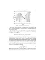
content of the waveforms. Fig. 6 presents the spectrum of the line-to-line supply voltage ob-
tained by FEM and analytical motor models incomparisonwith the measured spectrum,and
Fig.7presentsthecorrespondingresultsforthephasecurrent.Thefundamentalcomponents
are scaled out from the figures in order to see the differences in higher harmonics. Inthevolt-
age spectrum, distinctive difference is seen between the FEM model and analytical model
in certain frequencies, but otherwise they follow each other closely and also correspond
very well with the measured results. In the current spectrum, the difference between FEM
model and analytical model issignificant in all harmonic components. It isalso seen that the
currentspectrum obtained by the FEM model agreesvery well with the measured spectrum.
Good agreement between the simulated and measured results shows that the control
model behaves correctly in the simulations and the weak coupling between frequency
Figure 6. Spectrum of the supply voltage obtained by the FEM and analytical models and compared
with the measured spectrum.
I-8. Coupled FEM and System Simulator 89
Figure 7. Spectrum of the phase current obtained by the FEM and analytical models and compared
with the measured spectrum.
converter and FEM models gives correct and reliable results. Furthermore, the voltage

spectrum reveals that the analytical model is adequate for modeling the control system in
steady state, but the differences in the current spectrum clearly proves the better accuracy
of the FEM model over the analytical model in the harmonic analysis of the phase current.
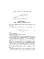
This is alsoillustrated in Fig.8, which presents theimpedance of the motor for the measured
frequency range. The impedance obtained by the FEM model follows closely the measure-
ments until 4 kHz, whereas the analytical model shows two times higher impedance at the
same frequency.
The measured losses of the motor in steady-state operation were 58.8 kW, and the losses
estimated by the FEM-based motor model were 60.6 kW, which shows excellent capability
Figure 8. Impedance of the motor obtained by the FEM model, analytical model, and measurements.
90 Kanerva et al.
Figure9. Electromagnetic torqueandphase currents, whenthe torqueischanged fromzerotonominal
and from nominal to 0.5 pu.
for loss prediction. In FEM, the copper losses in the coils were determined from the resis-
tance and current density, and the iron losses were determined from the harmonic compo-
nents of the supply voltage and the loss factors provided by the iron sheet manufacturer.
Transient operation using FEM model
Aftervalidatingthedrivesimulator with steady-state measurements, the drivewassimulated
in transient operation. A torque step from 0 to 1.0 pu was applied, when the motor was run-
ning at nominal speed. After a while, the torque was changed to0.5 pu. The electromagnetic
torque and the phase currents of the motor are presented in Fig. 9.
In another transient simulation, rotational speed was changed from nominal to 0.3 pu,
while operating at no load conditions. The inertia of the motor was reduced in order to have
a faster speed change. The electromagnetic torque and rotational speed are presented in
Fig. 10.
In both transient simulations, the control system responds well to reference changes. Al-
though notvalidated by measurements, the results showthe capability to simulate transients
of the controlled drive system.
Determination of the initial state
Traditionally,findingoutthecorrect initialstatefortheFEM computation has beenproblem-

atic. Especially with static frequency converter models, simulation of the startup transient
may take hours of computation time.Even if the simulation is started from an initial fieldob-
tained by sinusoidal supply, several periods of fundamental frequency must be time stepped,
until the transient has stabilized in the motor.
Inthepresentedsimulationenvironment,the initial transientconvergedremarkablyfaster
than in the previous studies. This is due to the calculated initial states for all state variables
I-8. Coupled FEM and System Simulator 91
Figure 10. Electromagnetic torque and rotational speed, when the speed reference was changed from
nominal to 0.3 pu.
and accurate closed-loop model of the control system, which estimates the magnetic state
of the motor and controls the supply voltage to set the motor in the required operating point
as quickly as possible. In other words, the simulation model operates exactly as the real
drive system.
Conclusion
This paper presents a drive simulator system comprising a three-level inverter, speed/torque
control by DTC algorithm and an analytical or FEM-based motor model. The FEM model
of the motor is coupled with SIMULINK using indirect approach. This means that different
parts of the drive system can be simulated simultaneously, but using different time steps.
An asynchronous machine drive was simulated using analytical and FEM-based motor
models and the results were compared with measurements. In the supply voltage spectrum,
agreement with measured results was excellent for both motor models. In the current spec-
trum, agreement with the measurements was clearly better with the FEM-based model.
In transient simulation, the control system responds very well to the changes in reference
values.
Using the proposed methodology, the FEM model of the motor and the frequency con-
verter model can be designed separately and easily combined for coupled simulation.
With the developed simulation environment, the initial states for the analytical motor
model and the FEM computation are achieved very rapidly. Based on the results, analytical
motor model is suitable for control design, but FEM model is needed for detailed analysis
of the saturation and frequency dependence of the motor parameters. As well, the motor

losses obtained by the FEM computation agree very wellwiththe measurements. In general,
the simulation results with the FEM model are very accurate and reliable, which leads to
benefits in the design and development of advanced control algorithms.
92 Kanerva et al.
References
[1] A. Arkkio, “Analysis of Induction Motors Based on the Numerical Solution of the Magnetic
Field and Circuit Equations”, Acta Polytechnica Scandinavica, Electrical Engineering Series,
No. 59, 1987, p. 97. Available at .fi/Diss/198X/isbn951226076X/.
[2] J. V¨a¨an¨anen, Circuit theoretical approach to couple two-dimensional finite element models with
external circuit equations, IEEE Trans. Magn., Vol. 32, No. 2, pp. 400–410, 1996.
[3] A.M. Oliveira, P. Kuo-Peng, N. Sadowski, M.S. de Andrade, J.P.A Bastos, A non-a priori ap-
proach to analyze electrical machines modeled by FEM connected to static converters, IEEE
Trans. Magn., Vol. 38, No. 2, pp. 933–936, 2002.
[4] S. Kanerva, S. Seman, A. Arkkio, “Simulation of Electric Drive Systems with Coupled Finite
Element Analysis and System Simulator”, 10th European Conference on Power Electronics and
Applications (EPE 2003), Toulouse, France, September 2–4, 2003.
I-9. AN INTUITIVE APPROACH TO
THE ANALYSIS OF TORQUE RIPPLE
IN INVERTER DRIVEN
INDUCTION MOTORS
¨
O. G¨ol
1
, G A. Capolino
2
and M. Poloujadoff
3
1
Electrical Machines and Drives Research Group, University of South Australia, Australia GPO Box
2471, Adelaide SA-5001, Australia

2
Energy Conversion and Intelligent Systems Laboratory, Universit´e de Picardie Jules Verne 33, rue
Saint Leu, 80039 Amiens Cedex 1, France

3
Universit´e de Pierre et Marie Currie—Case 252, 4 place jussieu, 75252 Paris, France

Abstract. An intuitive approach of parasitic effects with particular emphasis on torque ripple has
been proposed successfully. It is shown that a good approximation can be achieved in predicting the
nature and the magnitude of torque ripple by the use of a relatively simple time-domain model.
Introduction
It is well known that, when an induction motor is driven from a non-sinusoidal supply,
problems may arise due to the presence of supply harmonics. For instance it is well known
that the use of a six-step inverter may lead to the creation of parasitic effects such as torque
pulsations accompanied by noise and vibration. It is less well known that torque ripple
along with associated disturbances can also be present in the case of drive systems which
emulate a sine wave, such as field orientation control schemes if and when they are driven
into overmodulation.
Various methods of analysis have been proposed to assess the extent of the effect of
supplying a motor from a non-sinusoidal source [1–3]. Of these, methods which are based
on frequency domain analysis yield results which provide no interpretation of time-domain
results, thus notallowingthe significance ofsupply harmonics in terms ofparasitic behavior
to be appreciated when a harmonic-riddled source is used.
This paper proposes an intuitive approach to the analysis of parasitic effects with par-
ticular emphasis on torque ripple. The approach is based on the notion of space phasor
modeling [4]. It is shown that a good approximation can be achieved in predicting the
nature and the magnitude of torque ripple by the use of a relatively simple time-domain
model.
S. Wiak, M. Dems, K. Kom

˛
eza (eds.), Recent Developments of Electrical Drives, 93–100.
C

2006 Springer.
94 G¨ol et al.
Basic considerations
Both direct phase models [5] and orthogonal models (generally referred to as d-q models—
based on Park’s two reaction theory [6]) have been used in analyzing the time-domain
performance of asynchronous motors.The formerhave been considered to bemore relevant
to the modeling of polyphase machines since directly measurable physical quantities are
presentinthe modelandeffectsofwinding asymmetry andsupplyunbalancecanbeassessed
with relative ease. But the use of the latter has been far more pervasive.
On the other hand, it seems to have gone unnoticed that space phasor models offer
a valid and interesting alternative. They intrinsically contain the elements of both direct
phase models and orthogonal models, making the progressive or the retrogressive transition
between space phasor models and others possible. Furthermore they correctly model the
rotating field within the machine space. Thus their adoption for modeling may arguably
constitute an “intuitive” approach.
The space phasor concept
The transition from a direct phase model to a space phasor model can be effected by be-
stowing“vector”attributesupon the time-variantelectromagneticquantities of the machine.
Thus the sum of stator and rotor phase currents for a three-phase machine in space phasor
notation become
˜
I
S
=
2
3


I
SA
+
˜
aI
SB
+
˜
a
2
I
SC

(1)
˜
I
S
=
2
3

I
SA
+
˜
aI
SB
+
˜

a
2
I
SC

(2)
Stator phase voltages can also be expressed as a single space phasor quantity as
˜
U
S
=
2
3

U
SA
+
˜
aU
SB
+
˜
a
2
U
SC

(3)
Similar considerations apply to flux linkages, namely
˜

λ
S
=
2
3

λ
SA
+
˜
aλ
SC
+
˜
a
2
λ
SC

(4)
where
˜
a = e
j
2π
3
(5)
˜
a
2

= e
j
4π
3
(6)
It must be emphasized that the complex j-operator used in the definition of the unit
space phasors
˜
a and
˜
a
2
has a completely different connotation from the one used in
electrical circuit analysis: it designates a spatial shift of the quantity with which it is
associated.
Equations (1) to (4) imply that a single space phasor can be constructed on the basis of
individual phase windings of the polyphase motor. Alternatively, especially if the transition
is from a transformed model as in the case of orthogonal models, the aggregate stator and
I-9. Torque Ripple in Inverter Driven Induction Motors 95
rotor currents in space phasor notation can also be expressed as
˜
I
S
= I
α
+ jI
β
(7)
˜
I

R
= I
d
+ jI
q
(8)
Similar considerations apply to both the stator and rotor phase voltages and flux linkages,
namely
˜
U
S
= U
α
+ jU
β
(9)
˜
U
R
= U
d
+ jU
q
(10)
˜
λ
S
= λ
α
+ jλ

β
(11)
˜
λ
R
= λ
d
+ jλ
q
(12)
The machine model
With the foregoing considerations, a space phasor model describing the electromagnetic
behavior of the entire machine can be devised; remarkably, consisting of a single model
equation for stator and rotor phase windings respectively, that is
˜
U
S
= R
S
˜
I
S
+ p
˜
λ
S
(13)
˜
U
R

= R
R
˜
I
R
+ p
˜
λ
R
(14)
where
˜
U
R
= 0 for the singly excited induction motor.
In terms of electrical circuit model parameters the equations can also be written as
˜
U
S
= R
S
˜
I
S
+ L
S
p
˜
I
S

+
3m
2
pR
S
˜
I
R
(15)
0 = R
R
˜
I
R
+ L
!R

p
˜
I
R
+ jpϑ
˜
I
R

+
3m
2


p
˜
I
S
+ jpϑ
˜
I
S

(16)
Together with the equation of motion given below, this deceptively simple model can be
deployed to analyze the behavior of a polyphase induction motor in the time domain.
T
elec
= Jpω + Dω + T
load
(17)
In the above equations, p denotes the time derivative of the variable it precedes.
The electromagnetically developed torque can be obtained as:
T
elec
=
3m
2


˜
I
R
˜

I
∗
S

(18)
The supply model
If the induction motor is to be operated in a variable speed drive, then the non-sinusoidal
nature of the supply voltage must be taken into account in modeling the drive to reflect the
effect on machine performance of the harmonic content of the supply voltage. In the case
of a voltage source inverter configured in six-step mode, illustrated in Fig. 1, the terminal
voltages V
A
, V
B
, and V
C
are as depicted in Fig. 2. For the purposes of this discussion, the
inverter model shown here assumes ideal switches. Fig. 2 depicts the resultant voltages at
96 G¨ol et al.
V
A
V
C
A
B
C
H
E
V
B

E/2
E/2
Figure 1. Voltage source inverter.
V
B
V
C
E/2
E/2
E/2
V
A
Figure 2. Terminal inverter voltages.
the inverter terminals, leading to “six-step” voltages across the stator phase windings of the
motor.
The space phasor form of the resultant “six-step” voltage applied to the motor ter minal
can be conveniently obtained in terms of orthogonal components as
˜
U
S
= U
α
+ jU
β
(19)
U
α
(t) =

2

3

V
A
−
V
B
+ V
C
2

(20)
U
β
(t) =
1
√
2
(
V
B
− V
C
)
(21)
The Fourier expansions of U
α
and U
β
give

U
α
=

2
3
2E
π
∞

k=1
sin(2k −1)
π
6
+ sin(2k −1)
π
2
2k −1
cos(2k −1)ωt (22)
U
β
=
1
√
2
4E
π
∞

k=1

cos(2k −1)
π
6
2k −1
sin(2k −1)ωt (23)
Obviously, not all harmonics in (22) and (23) are significant in terms of causing parasitic
behavior.Onlythose har monics whicharesignificant andcanprofoundlyaffectperformance
need be considered in the supply model.