Gear Noise and Vibration Episode 1 Part 8 pdf

8
Recording
and
Storage
8.1
Is
recording required?
For
much work, especially
for
initial investigations
and
development,
there
is
little point
in
recording masses
of
data, whether T.E.
or
vibration.
Displaying
the
information
directly
on an
oscilloscope, preferably
triggered
to

synchronise with
I/rev
of
pinion
or
wheel
is
very valuable
and
should never
be
omitted.
It is
especially
useful
when
the
problem occurs
at
particular
points
in the
revolution.
A
typical example
is the
noise
of a
timing
drive

clatter
on a
diesel engine.
Even
more important
is the
information
from the raw
signal
to see
whether
noise
or
vibration
is due to
isolated impulses
or to
steady excitation.
Steady
vibration, typically
at
one-per-tooth
frequency, is
easily recorded
by
hand
since
the frequency is
obvious
and

there
is a
single Figure
for
amplitude.
A
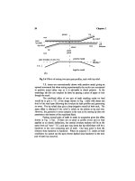
T.E. trace such
as
that sketched
in
Fig.
8.1
will give
an
immediate value
for
eccentricity
and for the
(expected)
1/tooth
so no
data logging
is
required,
whereas
a
trace such
as
that
in

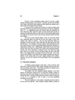
Fig.
8.2
needs recording
for
detailed analysis.
If
a
condition
is
transient
(e.g.,
scuffing)
or if
there
is a
suspicion that
a
small regular defect
is
hidden underneath steady
or
irregular vibration, then
it
is
essential
to
record
for
detailed subsequent analysis.
It is not

unknown
for
the
signal-to-noise
ratio
to be -20 dB (or
even lower)
in a
gearbox.
T.E.
1
rev
Fig
8.1
Simple T.E. trace.
121
122
Chapter
8
vel
1
rev
Fig 8.2
Complicated vibration recording.
"Noise"
in
this context
is
used
to

describe
any
electrical
or
mechanical
vibration which
is not the
vibration
of
interest.
8.2
Digital versus analog
Until
20
years
ago
analog
(tape)
recording completely dominated
the
field of
data recording. Digital storage
was
expensive
and
restricted
in
size
and
sampling rate,

so
there
was
virtually
no
competition
to 14,
16
or 32
track
recording
on
magnetic tape. Information rates
up to 300 kHz per
track were
possible, equivalent
on a 14
track recorder
to a
total digital sample rate
of
well
over
10
million
samples
per
second. Total storage times were
700
seconds (even

at the
highest data
rates)
so
equivalent memory capacity
was
huge.
A
disadvantage
of
analog recording
was
that
the
signal-to-noise
ratio
was
little better than
40 dB in
practice
so
that recording noise levels were
of
the
order
of 1% of the
signal.
In
this case
the

electrical noise
was due to the
magnetic recording process
and was
random
in
nature.
In
comparison,
the
standard
12 bit
digital
recording
has a
theoretical
effective
recording level
more than
70 dB
down, below 0.03%. This
is not
quite
the
advantage
it may
seem since
the
noise
floor

of the
(analog) equipment providing
the
signal
is
likely
to be
relatively high, perhaps about 0.5%. Analysis
of the
results
inevitably
involved replaying
the
analog signal into some
form
of
digital
analysis
equipment
so
that there
was an
extra transfer needed.
Current
tape
recorders
are a
hybrid since they typically record
on
video

cassettes
and can
record multiple tracks
at
high rates but, like
CD
players, they record
the
information
digitally.
To
replay, they convert
the
information
back into analog
form
and it is
then re-digitised
in a
computer
for
Recording
and
Storage
123
analysis.
Signal-to-noise
ratios
are
good since

the
information
is
stored
digitally.
However, such recorders
are
expensive
and
heavy.
With
the
advent
of
cheap active memory
and
very cheap digital
storage
the
situation
has now
changed completely
so
that nearly
all
recording
is
digital.
The
requirements

for
most gear noise
and
vibration work
are
relatively
modest. Necessary recording
frequencies are
limited since 1450
rpm
and 24
teeth
is
less than
600 Hz
tooth
frequency and we can
record
up to
the
5th
harmonic
of
this tooth
frequency
(giving
3
kHz) with
a 10 kHz
sampling

rate. This leads
us to
record directly into
a
standard (cheap)
PC or
portable (laptop) computer.
8.3
Current
PC
limits
Given
sufficient
expenditure there
are now few
limits
on
what
can be
achieved
digitally with
a
special purpose computer. However, prices rise very
rapidly
if we
depart
from
what
is
standard

and
easily available
so it is
advisable
to
tailor testing
to
current standard
PC
performance.
A
standard
PC
together with
a
basic
16-channel
12 bit
data logging
card
can
cost less than
£1000
($1500).
It is not
necessary
to use an
expensive
card with output capabilities
or

sophisticated facilities. This
will
allow total
sampling
rates
up to 200 kHz
(kilo
samples/sec)
and the
information
can be
poured (streamed) straight onto hard disc.
The
information
is in the
form
of
12
bit
samples
so
with direct storage each data point takes
up 2
bytes
of
memory.
A free
memory capacity
of 20
gigabyte

on the
hard disc allows
10,000
million samples
to be
stored
and
with
6
channels
at 10 kHz (60 kHz in
total)
the
recording time possible
is
160,000
sees
or 44
hours,
far
more time
than
is
needed
for a set of
tests
for
noise investigation
or
development

purposes.
If
condition monitoring
is
being investigated then
44
hours
is
likely
to
be
insufficient
and
techniques
are
needed
to
reduce
the
quantity
of
information
to be
stored.
Twelve
bit
resolution
(1
part
in

4096)
is
currently standard
and is a
good compromise. Eight
or 10 bit
resolution
is not
really
sufficient
when
the
signal contains
a
small vibration
of
interest, swamped
by a
large vibration
that
is
irrelevant. Sixteen
bit
resolution
is not
needed since, with
the
fairly
standard range
of ± 5 V,

each
bit
would
be
only
0.15
millivolts, well below
the
noise level. Resolution
or
discrimination, typically
2.4 mV for 12 bit
recording, should
not be
confused with accuracy which
is
usually about
1%
for
vibration, equivalent
to 100 mV for 10 V
full
scale.
In
general, absolute
accuracy
is not
important because
we are
looking

for
changes
or
differences.
Occasionally
it may be
worthwhile
to
consider double recording information,
124
Chapter
8
once with
all the
information present
and
then
in
parallel, cutting
out
irrelevant
high
or low frequency
information
with
a
filter
and
amplifying
to

give
just
the
information
of
interest.
For
data logging
on
site
the
same considerations apply, although
the
portable laptop computer
and the
necessary PCMCIA card
are
slightly more
expensive,
so the
cost approaches £1500 ($2000)
for up to 16
channels
at 200
kHz
total sampling rate.
It
is
tempting
to

consider streaming
the
test data straight onto
CD
instead
of
onto hard
disc
and
there
is
then
the
advantage
that
if
non-
rewriteable
discs
are
used there
is a
permanent very cheap archive.
With
a
storage capacity
of 650 MB or 300 M
samples
for
less than

£2
($3) storage
costs
are
negligible.
When
T.E.
is
being recorded
the
requirements
are for
perhaps
4
revs
at
1,000
samples
per rev
with
3
channels being recorded
so
each mesh check
requires only
24 kB of
storage.
One CD can
store
the

results
for
20,000
gear
checks.
8.4
Form
of
results
A
question
often
asked
is
whether vibration information should
be
recorded, analysed
or
stored
as
acceleration, velocity
or
displacement,
and
there
is
sometimes
frank
disbelief that
an

acceleration signal, when
integrated, provides
a
velocity signal.
Ci
input
accel
output
vel
Fig 8.3
Circuit
to
integrate acceleration
to
velocity.
Recording
and
Storage
125
Almost
exclusively,
the
original vibration measurement
is now
acceleration
but it is
easy
to
carry
out one

stage
of
integration
to
velocity,
as
in
Fig. 8.3, with
an
operational
amplifier.
The
basic integration
is the
input resistor
Rj
working
with
the
feedback
capacitor
C
2
but an
extra blocking capacitor
is
needed
at
input,
and

a
parallel resistor
R
2
in the
feedback,
to
prevent
drifting
to
saturation.
The
time
constants (RC)
for
input
and
feedback
should
be
kept larger than
the
value
of
(1/co)
for the
lowest
frequency to be
measured. Typically
the

combination
of an
input
Rj
of 100
kfi
and
C
2
of
0.01
^F
gives
a
time constant
of
integration
of 1
millisecond
so
that
if the
input scaling
is 1 V per m
s~
2
the
output
corresponds
to 1 V per mm

s"
1
.
At
input,
an
R
t
of 100
kQ
and
Ci
of
luF
gives
a low end
rolloff
frequency
of
10
rad/s
or 1.6 Hz and to
match this
with
C
2
of
0.01
uF
requires

an
R
2
of
10MD.
If
only audible
noise
matters, then
the
low-cut blocking
frequency can be set
fairly
high
at,
say,
30 Hz,
greatly reducing
drift
problems.
hi
theory
a
second
stage
of
integration, identical
to the first
stage
could

be
used
to
give displacement,
but in
practice this
is
rare.
The
double
integration
tends
to
give
a
rather unstable
fluctuating
signal which
floats
considerably since
the
slightest
spurious components
at low frequency in the
original
signal
are
greatly
amplified
by the

double integration. Using chopper
stabilised
instrumentation
amplifiers
helps
but
does
not
completely solve
the
problem
and may
inject chopper
frequency
noise.
Integration
can be
carried
out
digitally
on the
signal
but
suffers
from
the
same
drift
problems
as the

analog approach
and a
standard
PC
with
simple
software
cannot stream data
to
disc
and
integrate simultaneously.
If
double
integration
to
displacement
is
needed,
the
best compromise
is
usually
to
analog integrate
to
velocity, record velocity, then digitally integrate
to
displacement
and

then high-pass-filter
to cut out
spurious
low frequency
drifts.
A
convenient alternative
is to
record velocity
and to frequency
analyse
the
velocity signal then digitally divide each band amplitude
by the
angular
frequency to get the frequency
spectrum
for the
displacement.
Whether
acceleration, velocity
or
displacement should
be
recorded
depends
on the
engineering requirements.
For
noise purposes

it is
velocity
that
tends
to be
proportional
to
noise
and it is
also velocity that
is
most likely
to
remain roughly constant over
a
very broad range
of frequencies.
Hence,
for
noise
investigations
we
usually record (and analyse) velocity using
an
analog
integrator
to
avoid integrating digitally. This greatly reduces
the
danger

of
the
signal
of
interest
being
too
small, unlike
using
acceleration which
is
tiny
at
low frequencies or
displacement which
is
miniscule
at
high
frequencies.
126
Chapter
8
constant
velocity
region
limiting
displacement
region
limiting

acceleration
region
permissible
vibration levels
frequency
(log
scale)
Fig 8.4
Typical test
limit
vibration specification.
In
contrast, when positional accuracy matters
for
timing gears
or
printing,
the low frequency
components dominate
the
results
and it is
better
to
record displacement
(as
with T.E.).
For
monitoring,
the

troublesome
occurrences
exist
for
very short
time
scales
and
acceleration
is
preferred, emphasising
the
higher
frequency
components.
In
extreme
cases
it can be
worthwhile
to
consider recording
"jerk,"
the
differential
of
acceleration.
A
typical "customer acceptance vibration specification"
for a

gearbox
imposes
a
constant velocity
limit
(7.5
mm
s"
1
peak) over
the
central working
part
of the
range, then
goes
to
constant displacement
limit
(40
um
p-p)
at low
frequency and
nearly constant acceleration
limit
(50 - 100 m
s"
2
)

at
high
frequency
(see Fig. 8.4, which
is
typical
of the
AGMA
specification)
[1,2].
This type
of
approach tends
to
assume that
the
problems exist
at
well
separated
frequencies so the
separate
frequency
bands
do not
combine
to
generate
high peak values. This
is

usually relevant
for
noise,
but not
when
accuracy
is
involved, since
a
signal plus harmonics
can
give
a
peak value
many
times higher than
a
single component when pulses occur (see section
9.3).
It is
unfortunate that there
is no
easy method
of
substituting
for a
look
at the
original time trace
on an

oscilloscope. Humans
are
very good
at
detecting that something
is
different
or
"wrong" even though they
may not be
able
to
specify
the
problem exactly.
Recording
and
Storage
127
ampl
1
\f
\
II
/I
I
1
maxfreq
of
interest

N
'
1
1
i
i
i
i
1
1
1
r
i
i
i
i
i
t
20
Hz
T
sample
frequency
filter
characteristic
4kHz
5kHz
frequency
15kHz
Fig 8.5

Typical
frequency
ranges
for
data recording
and
sampling.
8.5
Aliasing
and
filters
There
is a
very large amount
of
literature about electrical
"noise"
problems
and
about
the
problems
of filtering,
sampling
and
aliasing.
Unfortunately
not all
that
is

written
is
necessarily correct when tackling
a
particular problem
and
high costs
can be
associated
with sophisticated
filters,
which
may be
redundant.
The first
essential
is to
decide
on the frequency
range
of
interest
and
a
standard conventional solution
is as
indicated
in
Fig. 8.5.
The

(audible)
frequencies
of
interest might
be 30 Hz to 4
kHz,
filters
(band pass
4 or 6
pole)
would
be set at
perhaps
20 Hz and 5
kHz,
and
sampling might
be at 15 kHz
(or
technically
15k
samples/sec).
The
sampling rate
and filtering are
interlinked. Sampling theory
[3]
says
that
we can

detect
a
signal
up to
half
the
sampling
frequency but the
effect
of
"aliasing"
is to
allow
false
indications
if
there
is
high vibration above
half
sampling
frequency. The
effect
is
sketched
in
Fig.
8.6 and
shows
how a

high
frequency
input
at
f
b
when sampled
at
f
s
,
can
appear
to be at a
frequency of
(fg
-
fi
).
This means that vibration above
fg/2
needs
to be filtered
out.
128
Chapter
8
. .
,
.

,
apparent sampled signal
onginal
signal
time
^~
•
sample points
Fig 8.6
Sketch
of
sampling giving
false
frequency.
The
effect
is
sometimes called
a
"picket
fence"
effect
and is
occasionally seen
in
very
old
films
where
car

wheels appear
to be
rotating
backwards.
It is the
same
effect
as
using
a
stroboscopic
flash
to
slow down
or
reverse
a
vibration
or
rotation.
The
resulting
frequency
spectrum
is
"reflected"
in the
output
spectrum
as if

there were
a
mirror
at frequency
f/2
(the "folding"
or
Nyquist
frequency) and it
means
that
a
high signal
at frequency 0.6
f
s
will appear
at a
frequency 0.4
f
s
,
as in
Fig. 8.7.
The
mathematics
of
Fourier
frequency
analysis with sampled

vibrations
cannot detect
the
difference
between
those
frequencies
above
C/2
and
those below. When
a
fundamental
frequency
analysis
is
carried out,
the
result gives both
the
components above
and
below
the
folding
frequency as
conjugate pairs
and we
arbitrarily (and sometimes incorrectly) assume that
it

is
solely
the
lower
frequency
that
is
there.
The job of the
band pass
filter
is to
make sure that
all frequency
components above
f/2 are
negligible
so
that they cannot influence
the
frequency
range
of
interest.
Filters
are not
perfect devices
and if we
take
the

standard (rather expensive)
four
pole
filter
it
will
have reduced amplitude
by
2
4
at
double
its
nominal
or
roll-off
frequency.
In
the
case
quoted above with
f
s
at
15
kHz,
a
spurious signal
at 10 kHz
would

be
reduced
to 6% of its
value
by
a
filter
set at 5 kHz and
would appear
to be at a frequency of
15
- 10,
i.e.,
5
kHz.
To
appear within
the frequency
range
of
importance,
< 4
kHz,
the
Recording
and
Storage
129
original vibration would have
to be at 15

-4,
i.e.,
11kHz,
and
would
be
reduced
by a
factor
of
(2.2)
4
(i.e.,
down
to
4.3%
of its
original value).
Filters with
a
higher roll-off rate than
the
standard
four
pole
filter
can be
used
but
they

may be
more expensive, more temperamental with
regard
to
"ringing"
when there
is an
impulse,
and may
give
"ripples"
of
non-
constant amplification
in the
passband.
ampl
actual frequency
response
"folding
frequency"
I
reflected
response
I
I
sample
frequency
I
fs/2

frequency
fs
Fig.
8.7
Aliasing
effect
in
sampled signal analysis.
For
general
testing
the
normal solution
is to
take
the top frequency of
interest
f^
set the
high
cut
filter
perhaps
25%
above
the top frequency, and
set the
sampling rate
to 4 x
fg.

The low cut
filter
is set
slightly below
the
lowest
frequency.
This
"standard"
solution tends
to be
applied without much
thought
to all
problems
and is
likely
to
result
in a
test setup that
is
unnecessarily expensive.
The set of
filters
may
easily cost more than
the
computer
and

data logging card
and be an
additional weight
to
carry
and
correspondingly increase equipment sales
profits
greatly.
The
first
casualty
of
actually using intelligence about
the filter
requirements
is the
need
for a
high performance (expensive) low-cut
filter at
the
bottom
end of the frequency
range.
A
simple blocking capacitor will
cut
off
DC

and,
especially
if we
record velocity,
the
time constants
of the
integrating
circuit
can be set to
reduce
the
I/rev components which,
in any
case, will
be
very small
for
both acceleration
and
velocity
and
will
be
ignored
in
the
final
assessment. This
one

change
can
halve
the
cost
of filtering as
130
Chapter
8
well
as
increasing reliability.
In one
very large industrial monitoring
installation, very expensive
low frequency filters
were used
to cut out
tidal
effects,
not
only greatly increasing
costs
but
removing
a
very
useful
permanent running check that
the

equipment
was
performing satisfactorily
with
regard
to
both timing
and
amplitude.
The
second casualty
can be the
need
for a
relatively high
performance
(4 or 8
pole)
filter at the top end of the frequency
range.
If
there
is
negligible vibration
at 12 kHz (to
appear aliased
as 3 kHz
when sampling
at
15

kHz) then
there
is
little point
in
spending money
to
attenuate
it and
either
a
simple
R-C first
order circuit
or a
relatively cheap
two
pole
filter can
be
used instead
of a
four-pole. This
is
very likely
to
occur
if
velocity
(or

audible
noise)
is
being
recorded
since
it is
unlikely that there
will
be
much
power
at 12
kHz, which
is an
ear-splitting
frequency.
The
third aspect which
can be
different
in the
particular
case
of
gear
noise investigations
and
checks
is the

permissible
frequency
range.
The
text
book approach
to
vibration analysis
may be
extremely worried that
"aliasing"
problems with, say,
a 10 kHz
sampling rate might mean that
a 6 kHz
vibration
is
wrongly identified
as a 4 kHz
vibration.
As far as
gearing
is
concerned, this
is
probably
not a
problem, since
if
1500

rpm
and 40
teeth give
a
tooth meshing
frequency of 1
kHz,
the
difference
between
4 kHz and 6 kHz
is the
(highly unimportant) difference between
the
4/tooth
and
6/tooth
harmonic
frequencies. As we are not
bothered
by
which harmonic
is
dominating
and our
prime concern
is to
know whether
or not
there

is a
high
harmonic
present,
we can
bend
the
rules
on frequency
range selection. This
allows
us
either
to use
much lower sampling rates than normal
or to put up
the
detection range relative
to a
"standard"
sampling rate.
In one
particular
gear monitoring problem
the
sampling
rate
was set at a
predetermined
10 kHz

so use of the
standard
approach would have limited
the
high
cut filter to
about
3
kHz.
The
high
cut filter was in
fact
set to 7 kHz so
that instead
of the
information being limited
to 3rd
harmonic
of
tooth
frequency
there
was a
very
useful
(if, technically, possibly incorrect) information recording
and
detecting
up

to 7th
harmonic. When replaying
it, the 7th
harmonic would show
as the
3rd,
and the 6th as the
4th,
but
this
was not
important
as the
objective
was
purely
to
detect trouble,
not to
identify
it
accurately.
When
a
compact (cheap) system
is
desirable
filter
chips
are

available
typically giving
a 5th
order
Butterworth
characteristic
and two
such
chips
can
be
cascaded
to
give high
rolloff
rates cheaply. They need
to be
driven
by a
TTL
oscillator such
as an
8038
at 100
times their required
rolloff
frequency.
There
is
also

a
limitation that
the
maximum input voltage
is
limited
to
about
4 V
when
the
rails
are at 5 V.
This requires that
an
input
signal
is
reduced
to
below
4 V, filtered
then re-amplified
to
return
to the
original size.
Recording
and
Storage

131
+5V
+15 V
output
BNC
Fig
8.8
Circuit
for
double
5th
order
low
pass
filter.
Such
a
circuit,
as
shown
in
Fig. 8.8,
is not
very accurate
for its
rolloff
frequency
and is
restricted
in its

performance
but is
sufficient
for
portable T.E. measurement purposes
and can
easily
be fitted
onto
a
standard
board
to
give
a
very compact unit
for
travelling.
There
is a
trade-off between
filter
performance
and
sampling rates
which
can
occasionally
be of
help

in
T.E. testing where there
is a
large
but
irrelevant additional signal present. With
the
high speed double-divide
system,
the
carrier
frequency
tends
to be fixed by the
requirement
to
give
enough
full
scale
to
accommodate eccentricities
in
less accurate
gears.
The
5th
harmonic
of
tooth

frequency
will also
be fixed and
there
may
then
be a
low
(< 3) frequency
margin between
the
harmonic
(at < 1 um
p-p)
and the
carrier
(at 400 um
p-p).
To
prevent aliasing when sampling
at
normal rates
requires attenuation greater than
60 dB but if the
sampling rate
is
increased
to
above
twice

the
carrier
fundamental
frequency the
carrier
will
appear
in the
final frequency
analysis
but
will
appear
at its
correct
frequency and so can be
ignored. This allows
the use of a
lower performance
and
hence more stable
132
Chapter
8
filter
which
is
less prone
to
ringing

or the use of a
much reduced
frequency
margin
between harmonic
and
carrier.
8.6
Information compression
Although
modern
PCs
have relatively large
(tens
of
gigabytes) hard
disc memories
and the
initial
investigations
of a
problem
will
require
raw
vibration
data, established routine testing does
not
wish
to be

overwhelmed
with
irrelevant data, especially where noise
is
concerned, since most audible
noise
is a
steady
or
repetitive phenomenon.
Depending
on the
type
of
problem there
are
several ways
of
reducing
the
sheer volume
of
data
but the
most
useful
method
is
time averaging
at

once
per
revolution (see section 9.5). This
is a
technique which
is
especially
relevant
for
rotating machinery.
We
select
a
particular
shaft
and,
for a
large
number
of
revolutions, average
the
vibration signal over
the
revolutions
so
that only vibrations
associated
with that
shaft

remain,
as all
other non-
synchronous vibration (and electrical
noise)
has
averaged
to
zero. Displaying
the
vibration
on an
oscilloscope synchronised
to
once
per rev has
much
the
same
effect
since
we
tend
to
average
out
visually what
we see on the
screen.
If

we
have
a
standard 1500
rpm
motor driving
a 24
tooth pinion meshing
with
a 119
tooth wheel, then
we
must complete
119
revs
of the
pinion
to
complete
a
meshing cycle,
and all
subsequent meshing cycles should
be
identical
so
there
is no
point
in

measuring
any
more complete meshing cycles
since
the
same information should appear again
and
again. This will take
4.76 seconds
for the
cycle,
and
with tooth
frequency 600 Hz and a
requirement
to
measure
up to 7th
harmonic
we
would sample
at
perhaps
16
kHz.
A
complete meshing cycle
is
then
76,160

data points
for
each
of the
channels recorded.
At
the
operating
speed,
a
single revolution
of the
pinion
(40
milliseconds) corresponds
to 640
data samples
and a
single revolution
of the
wheel
corresponds
to
3173
samples. Since
all the
information relevant
to the
complete meshing cycle
can be

stored
as one
averaged revolution
of the
pinion
and one of the
wheel,
we
only need
to
store
3813
items
of
information
instead
of
76,160.
Any
other method
of
storing
all the
information
relevant
to a
complete meshing cycle either requires much more storage
or is
much
less

accurate.
It is
usually assumed that storing vibration information
as a
frequency
analysis
is
much more compact than storing
the
original
raw
information,
but
this
is not
correct
for the
semi-repetitive
information
we get
with
machinery.
It is
only
correct
if
debatable assumptions
are
made about
a

stationary noise spectrum
[3].
Recording
and
Storage
133
arnpl
Fig.
8.9
Rectification
of
vibration signal.
Another possibility
for
information compression
arises
when
we
already know that
the
signal consists
of a
limited number (usually just one)
of
(known)
frequencies. We can
then
use
"enveloping"
techniques

which give
us the
overall amplitude
of
vibration without bothering with
the
detail
of
each
individual
cycle.
The
sampling rates needed
for the
envelope
are
much lower
than
for the
original vibration.
out
ground
ampl
Fig.
8.10
Former method
of
enveloping
vibration
signal.

134
Chapter
8
rectified
signal
ampl
Fig.
8.11
Preferable method
of
enveloping.
This type
of
information
may be
relevant
for
looking
at
I/tooth
frequency and its
modulation
due to
varying misalignment
or
torque
effects
or
looking
at

high
frequencies
when damage monitoring
as the
ringing
of an
accelerometer
may be
triggered
by
metal
to
metal contact (see Chapter
15)
Fig.
8.9
shows
how the
vibration signal,
at a
single
frequency,
symmetrical
about zero,
is
rectified ready
for
"enveloping."
Originally this
was

done,
as
shown
in
Fig. 8.10, with
a
diode charging
a
capacitor which
decayed relatively slowly.
Unfortunately
this method
is
insensitive
and is
very non-linear
and
may
hide subsequent small half cycles
as
sketched.
It is
much better
to
rectify
the
signal properly
and to
pass
the

rectified signal through
a low
pass
filter to
give
the
effect
which
is
shown
in
Fig.
8.11.
Peak amplitudes
are
reduced
by a
factor
of
n
but it is
easy
to
compensate
for
this
in the low
pass
filter.
As

diodes have non-perfect characteristics
it is
advisable
to use the
rather
odd
circuit shown
in
Fig.
8.12
for
rectification
as
this circuit greatly
reduces
the
effects
of
diode imperfections.
Care
is
needed
to use
suitably
fast
diodes
at low
impedances
to
achieve satisfactory performance

at
high
frequencies and low
amplitudes.
The
advantage
of the
envelope approach
is
that
if
there
is a
vibration
frequency
of
interest
at,
say,
30 kHz
then
we
would have
to
sample
at a
rate
of
at
least

100 kHz to
catch this
frequency,
using
all the
available sampling rate
with
a
basic
PC and
board. Typically with rectification
and
smoothing,
the
low
pass
filter may be set to
about
2 kHz and a
recording sampling rate
of 3
kHz
would
be
satisfactory, despite
the
normal sampling rules quoted
in
textbooks.
Recording

and
Storage
135
output
input
Fig
8.12 Circuit
for
accurate rectification
of
small signal.
The
standard sampling
rules
do not
seem
to
apply
for
problems such
as
this where
the
main requirement
is to
have
the
area under
the
envelope

roughly
right. Practical testing with
an
artificially
generated signal with
bursts
of
perhaps
six
cycles
of
vibration
and
testing
by
varying
filter
frequency
will
give
a
very clear visible check
on
what
frequencies of
rolloff
and
sampling
are
satisfactory. Such

a
test signal
can be
obtained
by
(analog
or
digital) multiplying
a
single sided square wave
by the
carrier
(30
kHz)
to
give
a
test signal similar
to the
expected signal.
The
resulting reduction
in
sampling
rate and, hence, data storage
due to
enveloping
is
typically
at

least
30:1.
Another possible method
of
reducing information storage
is to
take
advantage
of the
known
form
of the
structure
of a frequency
analysis
of a
repetitive
waveform
such
as
that
from a
gear set.
We
know that
as the
waveform
is
repetitive there
can

only
be frequencies at
exact multiples
of
once
per
revolution
and
that
for
most gears with whine noise problems
it is
only
the
1/tooth
frequencies and
harmonics that
are
relevant. There
is
then
no
point
in
recording amplitudes
of all frequencies from the
Fourier analysis
as
there
are

only perhaps
five frequencies
that
are
relevant
for a
typical back
axle whine.
In
section
9.3 the
possibility
of
amalgamating several lines
from a
frequency
analysis
of a
T.E. record
is
mentioned
as an aid to
having
a
clearer
assessment
of the
total power
in the
region

of a
tooth
frequency or
harmonic.
This also reduces
the
amount
of
information stored
(by a
factor
of 10) if it is
being stored
in the
form
of a frequency
table.
136
Chapter
8
8.7
Archive information
The
problem
of
archiving
is
linked
to the
problems

of
data
compression.
The
normal (cheap)
PC
hard disc currently
has
perhaps
20
gigabytes
of
space
left
free
after
allowing
for
programs
so it can
store
up to
about
30
hours
of
information
for, say,
8
channels each

at 10
kHz. This
capacity
can be
reached
fairly
quickly
either
if
extended running
is
required
for
damage
monitoring
tests,
or if
production monitoring
is
required with
reasonable numbers
of
gears
being made.
After
the
initial
check
on the
results,

it is
very unlikely that
the raw
information
will
ever
be
required again
so it is not
necessary
to
have
the
information
readily accessible.
The
standard
CD at 650 MB
will
only store
about
1
hour's test results
for a
combined rate
of 80 kHz and so a
large
number
would
be

required
for
extended testing.
DVD
discs
will
store larger
quantities
but are not in
general
use yet and
formats have
not
standardised.
A
suitable compromise
for
vibration work
or
T.E.
tests
is to
store
selected
small
files
such
as the
most interesting mesh cycle averaged
files (as

in
section 8.6).
These
averaged
files
contain typically less than
4 k
points
and
so are
only
8 kB,
allowing noise test results
from
thousands
of
tests
to be
stored
on a CD
Rom, easily accessible
for
quick checks.
The
problem
is
then whether
or not to
bother
storing

the
original
raw
data which takes
up
perhaps
10 MB per
test,
just
in
case
there
are
strange
intermittent irregularities
in the
results which
do not
necessarily appear
in the
averaged
traces.
Caution suggests that, like taking
out
insurance,
the
information
should
be
archived just

to
ensure that
it
will
never, ever,
be
needed. Most
PC
systems have some
form
of
backup
and
typically
650 MB
backup
costs
less than
£2.
Since
it is
wise
to
have such
a
system
to
backup
the 400 MB of
software

on a
computer,
it is
also wise
to use it for
archiving
test data.
It
does
not
matter whether
the CD
writer
is fitted
internally
or, as is
more
likely
with
a
laptop, externally
via
USB.
It
is
worthwhile using non-
rewriteable
CDs to
remove
the

temptation
to
reuse discs
as
well
as
this being
more
economical.
There
are
much more elaborate, very high capacity backup systems
usually
based
on
tape drives
but it is not
worthwhile installing
a
system solely
for
archiving test
records.
Linked
to the
problem
of
generating archives
in the first
place

is the
almost
impossible problem
of
deciding when information should
be
scrapped.
There
is
little point
in
storing
information
on
gears
which have already worn
out but it is
extremely
difficult
to
take
a
decision
on the
time scale
for
killing
off
old
records. This

is one
problem
to
which
there
is no
satisfactory solution
but
the
more compact
the
storage
the
longer
can the
decision
be
delayed.
Recording
and
Storage
137
References
1.
American Gear Manufacturers' Association.
AGMA
Standard 6000-
A88.
2.
Dudley, D.W., Dudleys Gear Handbook,

Ch 13
Gear vibration,
McGraw-Hill,
New
York,
1992.
3.
Newland, D.E.N., Random vibrations, spectral
and
wavelet
analysis. Longman,
Harlow,
UK and
Wiley,
New
York, 1993.
Analysis
Techniques
9.1
Types
of
noise
and
irritation
One of the
most
difficult
problems
in

gear noise investigations
is
that
the final
"detector"
and
arbiter
(on
whether
or not a
noise
is
irritating)
is an
extremely
non-linear, rather temperamental,
and
extremely variable human
being, with
office
politics
and
economics playing
a
major
role.
It is
quite
possible
for

three
people
to
listen
to a
gear drive
and to
object
to it for
three
completely
different
reasons.
No
amount
of
technical measurement
will
determine which aspect
of a
gear drive noise
will
irritate
a
particular
customer,
so it is
most important
to
identify

the
problem correctly
at the
start
by
questioning
the
customer thoroughly
and by
possibly playing tapes
of
different
types
of
gear noise
to the
customer
for
comparisons.
A PC
with
an
output
card
to a
loudspeaker
can be
useful
for
this.

There are, roughly speaking,
four
types
of
irritation:
(a) A
steady tone. This
is
relatively musical and, because there
are few
harmonics, sounds
a bit
like
an
oboe.
It is
often
encountered
as a
"back axle whine"
on
rear wheel drive cars
and is
typically
in the 500 -
1000
Hz
range (900
rpm
and 40

teeth).
A
higher harmonic content
moves
the
character towards
a
stringed instrument sound.
(b) A
modulated tone. Here
the
customer
is not
objecting
to the
steady
component
at
perhaps
400 Hz but to the
fact
that
it is
modulated
(or
wowing)
at a
much lower
frequency. It is not
uncommon

to
have
a
customer complaining that
he is
hearing
a
noise
at 2 or 3
cycles
a
second. This
is
impossible. What
is
heard
is the
basic
400 Hz
once-
per-tooth
noise being modulated
in
amplitude
(or
phase)
at 2 or
3Hz.
(c)
I/rev

impulses. This
is the
type
of
noise generated
by a
defect
such
as
a
nick
or
burr giving
an
impulse
at
I/rev
and is
usually most noticeable
at
low
speeds.
The
sound
is a
fast
ticking sound
and has
very little
power associated with

it so it
will
not
usually show
up in a frequency
analysis. However, like
a
triangle
in an
orchestra,
it can
easily
be
picked
out by the
peculiar non-linear abilities
of the
human ear.
(d)
Grumbling
or
graunching.
This
is the
"classic"
gearbox noise, usually
associated
with
low
speed

and
heavily loaded drives.
It is the
typical
"bottom
gear"
noise
in a
car.
It
tends
to be
associated with pitch errors
and
is
essentially
at all
harmonics
of
once
per
revolution
of
both wheel
139