Gear Noise and Vibration Episode 2 Part 3 pot
Bạn đang xem bản rút gọn của tài liệu. Xem và tải ngay bản đầy đủ của tài liệu tại đây (867.59 KB, 20 trang )
180
Chapter
10
rubber
auxiliary
mass
main
mass
support
stiffnesses
I
\
original
response
ampl.
response
with tuned
damped
absorber
frequency
Fig
10.7
Tuned damped vibration absorber response.
Although
it is
possible
in
theory
to use
steel springs
and oil
damping,
this
is
rare
due to
sealing
and
tuning problems.
The
device needs
careftil
tuning
to the
correct
frequency and is, in
general,
only worthwhile
if the
auxiliary mass
can be
about
10% of the
effective
mass
of the
resonance
and the
original dynamic
amplification
factor
(Q) of the
resonance
was
greater than
8. The
absorber
can
then reduce
the Q
factor
to
below
4.
Improvements
181
Untuned
(Lanchester)
dampers which
use
only mass
and
viscous
damping
will work over
a
range
of frequencies but
require greater mass
and
give
much less damping
so
they
are
little used except
for
torsional engine
vibrations
which
occur over
a
wide range
of frequencies as
speed varies.
10.8 Production control options
When
trouble strikes
and the
customer's installation cannot
be
altered
there
is a
tendency
to
panic
and to
halve
all
drawing tolerances
on
principle,
to
make
sure that
all the
gears
are
being made
"better."
This
is, of
course,
no
help
if it is a
faulty
gear design
(or
installation)
and is
very expensive
to
achieve.
On
the
assumption that development
has
investigated permissible
loaded
T.E.
and
found
that
it
must
be
kept below, say,
4 um at
once-per-tooth,
there
are
several options available.
The
first
is the
obvious
one to run a
model
and
to see how
tolerant
the
design
is to
errors
of
profile, helix
and
pitch. This
should
give
a
good idea
of the
sensitivity
of the
design which could decide
how
tightly
manufacturing tolerances should
be
specified.
If
these tolerances
are
not
economically sensible then
the
choices
are:
(a)
alter
the
design
to
make
it
less sensitive
(if
possible);
(b)
greatly reduce tolerances;
or
(c)
manufacture
scrap.
Option
(b), though
often
used,
is
usually
far too
expensive. Option
(c), deliberately catering
for a
percentage
of
scrap,
is
guaranteed
to
produce
acute hysteria with production directors
and
accountants. However,
it is
surprisingly
often
the
most economic solution
and is
politically permissible
provided
that
the
small percentage
of
noisy boxes
are not
allowed
to go to the
customer. This means 100% T.E. checking
on the
production line.
This suggestion
of
100% T.E. production checking seems expensive
but
may
actually save money because some
of the
earlier checks
on
profile
and
pitch
can be
reduced
or
eliminated since detailed
faults
or
changes
will
be
picked
up by the
T.E. check. There
is
also
a
large hidden bonus,
due to the
statistics
of the
process,
provided that
a
pair
of
mating gears
are
checked
as a
pair,
not
separately
against
"master"
gears
which these days
may
well
be
little
more
accurate than
the
gears
they
are
meant
to be
testing.
If
gears
are
checked individually
for a
total error band
of 4 um in the
mesh then each gear must individually
be
within
+/- 2 um to
ensure that
any
pair
are
within
4 um.
This could well generate scrap rates
of the
order
of
10%
on
wheel
and
pinion.
Testing together will greatly reduce
the
scrap rate,
as
indicated
in
Fig.
10.8
since,
of the
"scrap"
pinions, most
of
those
"negative"
will encounter
wheels which
are not too
large
and
will mate satisfactorily.
182
Chapter
10
pinion
scrap
pass
max
permitted
difference
is T
pass
scrap
C
size
wheel
scrap
pass
pass
scrap
A
production
- T/2
limits
+ T/2
size
Fig
10.8 Combination
of
tolerance
limits
with gear pair testing showing
how
the
number
of
failed
gears
is
greatly reduced.
A
wheel
of
size
A
(which must
be
scrapped
if
tested separately) will
mate perfectly with
a
pinion
of
size
B, and
with
any
pinion
of a
size less than
C,
covering about
75% of the
pinions manufactured. This
effect
can
easily
reduce scrap rates
by a
factor
of
four
with corresponding savings.
The
cost
of
T.E. checking
is
relatively low.
The
standard commercial
checker
can
cost
up to
$300,000
(£200,000),
much
the
same
as a
profile, helix
or
pitch checker
but the
testing
is
very
fast
(it can
easily
be < 1
minute)
so
throughput
is
high, reducing costs.
Alternatively,
a
dedicated check
rig can be set up for a
standard
component such
as a
back axle.
The
cost
of the
mechanics, encoders
and
electronics
is
then
of the
order
of
$30,000 (£20,000) since
all the
high
precision slides
and
variable settings
of the
general purpose equipment
are not
needed.
There
is one
hazard which sometimes causes puzzlement when gear
design
is
improved
and
that
is the
oddity that
the
statistical
scatter
on the
final
noise levels
is
increased.
A
poor
and
rather noisy design might give
a
Improvements
183
measured noise level variation
of ± 2 dB.
When
the
design
is
improved,
the
variation
can
easily rise
to ± 5 dB so the
customer
may
complain about greater
inconsistency
in the
gear noise
and
assume that quality control
has
deteriorated.
The
reason
for
this
is
that
the
variations
in
T.E.
are
mainly
due to
manufacturing
so
they will stay roughly constant
at,
say,
± 2 um. A
poor
design
might give
a
fairly
regular
"design"
T.E.
of 8 um so ±2 um
gives
6 to
10
um, a
range
of
roughly
4 dB.
Improvement
of the
average T.E.
to 4 um,
still subject
to ± 2
urn
variation gives
a
range
of 2 to 6 um or a
total range
of
10
dB.
This manufacturing range cannot
be
reduced
by the
improved design
so the
customer
has to be
educated.
It is
difficult
to
convince
a
customer that
the
better
the
basic design,
the
larger
the
statistical variation
will
appear
to be.
The
ultimate
case
is
when
the
design
is
good enough
to
occasionally
(accidentally/miraculously)
give zero T.E.
and the dB
range
(at a
given
frequency) is
then infinite, regardless
of how
quiet
the
average gear pair
is.
References
1.
Fahy,
FJ.
Sound
and
Structural Vibration. Academic Press, London,
1993.
2.
Maag Gear Handbook, Maag, Zurich, 1990
(in
English), section
5.271.
3. DIN
3963, Tolerances
for
cylindrical gear
teeth,
(in
English),
DIN
standards, Beuth
Verlag
GmbH, Berlin
30.
4.
Smith, J.D.,
'Gear
Transmission Error Accuracy with Small Rotary
Encoders,'
Proc.
Inst.
Mech. Eng., Vol. 201,
No. C2,
1987,
pp
133-
135.
5.
Den
Hartog,
J.P.,
'Mechanical
Vibrations.',
Dover,
New
York, 1985,
Section
3.3.
Lightly Loaded Gears
11.1
Measurement problems
The
first
hint that
a
gear drive
may be
"lightly
loaded"
usually comes
when
vibration
or
noise measurements
do not
make sense. Amplitudes vary
for
no
apparent reason,
frequencies
appear which bear
no
relation
to
tooth
frequency
or
the
"phantom"
frequency
(from
the
gear
manufacturing machine)
and, most characteristic
of
all,
the
vibration levels
are
extremely dependent
on
load
levels.
The
standard response
of
taking
a
test
run and
doing
an FFT
analysis
just
produces even more
confusion
as the
signal gives roughly equal amplitudes
at
all frequencies and
appears
to be
trying
to
approximate
to
white
noise.
There
may be
stronger components near tooth
frequency and
harmonics
but
there
is a
high background continuous spectrum right through
the
range.
Even
worse, there
may be
significant
peaks
at
half tooth
frequency and
half
phantom
frequency or at
other
subharmonics
of the
obvious
frequencies, or at
curious
ratios such
as
two-thirds
of the
tooth meshing
frequency.
Since
all the
rules
of
linear vibration
are
being broken,
the
obvious
deduction
is
that
the
vibration
is
non-linear
and
that application
of
intelligence
rather than mathematics
may be
required.
Since
all frequency
analysis
is
based
on
the
assumption
of
linearity,
it is
hardly surprising that non-linear systems
cause
trouble since most vibration engineers have been brainwashed
(at
university)
into carrying
out an FFT
before
they start thinking.
The first
question usually asked
is
"what
do you
mean
by
lightly
loaded?"
This
is
best answered
by
saying that when
the
angular
accelerations
of
the
system multiplied
by the
effective
moment
of
inertia
exceed
the
steady
load torque,
which
is
trying
to
keep
the
teeth together, then
the
teeth
will
start
losing contact since
the
dynamic component
is
greater than
the
mean torque
level.
This
can
occur when
the
angular accelerations (due
to
T.E.
or
torsional vibration)
are
high,
the
moment
of
inertia
is
high
or the
load torque
is
low.
This
is
analogous
to
driving very
fast
over
a
bumpy road when (above
a
critical
speed)
a
lightly loaded trailer will start leaving
the
ground.
185
186
Chapter
11
A?
/\
A
/\
\
w
v
/\
/\
A
>V
/\
\/
V
v
/\
_
A
/x.
A
rx
y^\
—^"^y
\y
\
/
x
/
'
one
revolution
Fig
11.1
Vibration
on
successive revolutions
of
gear.
Lightly
Loaded
Gears
187
The first
essential with
a
non-linear
(or
linear) system
is to
look
at the
raw
vibration
(or
noise) signal
on the
oscilloscope,
preferably synchronised
to
once
per
rev. With recorded
traces
the
same
effect
can be
obtained
by
displaying perhaps
10
revs
in
succession
staggered
down
the
page like
a
waterfall
plot
as in
Fig.
11.1.
As
always
it is
very worthwhile having
a
I/rev
probe
to
give
an
exact synchronising signal.
11.2
Effects
and
identification
As
mentioned previously, humans
are
good
at
averaging viewed
signals
on an
oscilloscope
or the
same
effect
comes
from
time averaging
the
signal
so the
regular part
of the
pattern
can be
seen.
In
many
cases
a
human
is
better than
a
computer
for
seeing
what
is
happening.
In
one
engine test
in an
anechoic chamber,
at
idling,
the
timing train
was
extremely noisy
and FFT
analysis
of the
output
from a
microphone gave
apparently pure white
noise
with
no
individual
frequency
peaks,
much
to the
puzzlement
of the
team
of
development engineers.
The
installation
was so
elaborate (and extremely expensive) that
a
request
for a
look
at the
original
time signal caused dismay because
it was not
available. However,
after
an
hour's hard work
the
relevant signal
was
located
and
brought
out to a
simple
oscilloscope together with
a
I/rev
pulse. Once
the
signal
had
been
synchronised
on the
display,
no
explanatory words were needed
and the
dominating
sound
was of
heads being banged against walls.
The
time signal
was as
sketched
in
Fig.
11.2.
A
~
\J
V
w
time
one
revolution
Fig
11.2 Time trace
of
vibration synchronised
to
once
per
rev.
188
Chapter
11
The
time signal
not
only showed clearly what
was
happening
in
this
case
but
showed exactly where
in the
revolution
the
large engine torsionals
were acting
to
bring
the
timing gear teeth back into contact impulsively.
The
fundamental
frequency,
2/rev, about
25 Hz, was too low to be
picked
up
powerfully
by
microphone
or
accelerometer
so it was
solely
the
high harmonics
(with
much modulation) that dominated
the
measurements.
As far as
frequency
analysis
is
concerned there
is no
difference
between amplitude
distributions
for
white noise
and for
isolated short impulses (see section 9.3).
Both
distributions
contain equal amplitudes
at all frequencies and the
only
difference
is in the
phase synchronisation
at the
pulse.
More commonly,
the
torsional excitation
is due to the
T.E.
so
there
is
a
likelihood
of an
impulsive vibration
at
about
1/tooth
frequency,
varying
in
amplitude
and
period.
The
mechanism (Fig.
11.3)
is
similar
to
bouncing
a
ball
on
a
tennis racket
or
driving over
a
very
bumpy
road
at
high
speed.
A
short
and
rather violent impact
is
followed
by a
"flight"
out of
contact
until
the
load
torque
(or
gravity) brings
the
teeth back into contact
after
about
one
cycle
of
T.E. excitation.
It is
perfectly possible
to
bounce
powerfully
enough
to
land
2
or
3
cycles later
and we
then have
the
"subharmonic"
phenomenon
of an
excitation
at
1/tooth
giving
an
irregular vibration
at
once
per 2
teeth
or
once
per 3
teeth.
It is
difficult
for the
bounce
to
maintain consistent time
and
this
gives
a
very irregular variation
in
bounce height.
It
may
seem strange that
an
excitation
as
small
as
T.E.
can
give
trouble,
but
feeding
in a few
typical figures shows what
is
involved.
A
T.E.
of
±
5
um
(0.2 mil)
at a
I/tooth
frequency of
1000
Hz
corresponds
to an
acceleration
of 5
E-6*(6283)
2
which
is
roughly
200
m/s
2
or 20 g.
bouncing
response
ampl
input vibration
(T.E.)
Fig
11.3
Impulsive
bouncing response
to
roughly sinusoidal input.
Lightly Loaded Gears
189
A
pinion
of
mass
20 kg
will have
an
effective
linear mass
J/r
2
at
pitch
radius
of
about
10
kg so to
keep
the
teeth
in
contact requires
a
load
of
about
2000
N
(450
Ibf)
which
at
O.lm
radius
is 200 N m
(150
Ib
ft).
This
is
easily achieved
in a
normal loaded gearbox but,
in a
machine such
as a
printing machine,
20 g
acceleration
on a
printing
roll
with
an
effective
mass
of
500 kg
would require
10
tons tooth
load,
and the
load
due to
printing
is at
least
an
order lower than this,
so it is
difficult
to
keep teeth
in
contact.
Testing
with
portable high speed T.E. equipment
on a
printing
machine
will
show
the
manufacturing
gear
errors
repeating consistently
at low
speeds
but as the
speed rises
the
observed T.E. becomes erratic
and the
drive
can be
seen bouncing
out of
contact
for
long periods.
From
an
understanding
of the
basic mechanism
it is
soon clear that
varying
the
load
on the
system will have
a
major
effect
on the
vibration
and the
quickest
and
most telling test
for
non-linearity
is to
vary
the
load. This
may
mean
temporarily braking
the
driven component
to
increase
the
torque despite
the
power waste involved. Major changes
in
vibration immediately indicate
non-linearity whereas
minor
(<30%) changes suggest
a
linear system.
Curiously, both increasing
and
decreasing
the
load
may
make
the
system
better.
If the
vibration becomes worse, then usually
the
alternative
will
improve
it.
11.3 Simple predictions
As
with
all
problems
it
helps
to
have
a
simple model
of
what
is
happening
to see
what
the
effects
of
varying
the
parameters
are
likely
to be.
The
methods using
a
full
computer time-marching approach
as
described
in
chapter
5 are
necessary
if we
wish
to
detail
the
effects
of
misalignment, profile,
crowning, etc.,
in a
multi-degree
of freedom
system. Simple systems
can be
looked
at
rather quickly
by
making some very basic assumptions.
The
simplest
possible model
is the
single degree
of freedom
system
shown
in
Fig.
11.4.
The
response
of
this system
will
have
the
shape shown
in
Fig.
11.5.
The
torsional moment
of
inertia
has
been turned into
an
equivalent
"linear"
mass.
Due to the
non-linearity,
any
original narrow resonance widens
as the
resonance bends
to the
left
at
high amplitude.
Contact will
be
lost initially when
F =
myo
,
where
y is the
vibration
of
the
mass.
The
response above this
frequency is
generally unstable
and
erratic
but we can
make some estimates
for the
condition
of
maximum
amplitude
just
before
the
downward jump.
We
make
the
assumption that there
are no
energy losses during
the
"flight"
so
that
the
initial
"upward"
velocity
is the
same
as the
final
"downward" velocity.
190
Chapter
11
input
vibration
Fig
11.4 Simple model
of
non-linear system.
downward jump
as
frequency
decreases
upward jump
as
frequency increases
frequency
Fig
11.5
Response
of
"bouncing"
system
as frequency
varies.
Taking
the
coefficient
of
restitution
at the
short impact
as e and the
"landing"
velocity
as V
then,
as the
maximum upward velocity
of the
"base"
is
hco
(where
h is the
amplitude
of
vibration
of the
base),
the
relative velocity
after
impact must
be e
times
the
relative velocity before impact:
(V
-
hco)
= e (V +
hco)
Lightly Loaded Gears
191
During
the
flight
time there will
be a
constant restoring
force
F due
to the
load torque
so the
acceleration downwards will
be F/m
and,
since
flight
time
equals periodic time
2Vm/F
=
27t/co
Solving gives
o>
and V and the
bounce height will
be
mVV2F.
The
value
of
G>
will
be
less
than
the
value
at the
upward jump which
is
roughly
(F/m
h
)
05
.
A
slightly more refined version
of
this approach allows
for the
time
in
contact
for the
impact
as
this reduces
the
"flight"
time.
If the
contact
stiffness
is k
then half
a
cycle
of
contact vibration occurs
in
time
n
(m/k)°
5
so the
second equation becomes
05
27t/(D
-
7t
(m/k)
-
2 V
m/F
The
biggest uncertainty occurs with
the
value
of the
coefficient
of
restitution
at
impact
since
effective
masses
are
known. Once
the
impact
velocity
V and the
contact (tooth)
stiffness
are
known,
the
peak
force
can be
estimated since
by
energy
0.5mV
2
= 0.5
kx
2
where
x is the
maximum interference
and the
force
is k x. For the first
subharmonic
response
the flight
time
will
correspond
to two
periods (i.e.,
4
Tt/oo)
less
the
contact time.
One
danger with loss
of
contact
is the
possibility that
the
height
of
bounce
is
large enough
to
travel right across
the
backlash
and
impact
on the
unloaded trailing
flank. A
check
on the
meshing geometry
of a
standard spur
gear pair shows that,
as
might have been predicted
by the law of
general
cussedness,
the
impact
on the
trailing
flank
occurs
at a
time
to
inject
a
high
return velocity
and
there
is
liable
to be an
extremely destructive hammer across
the
backlash. Fortunately this
effect
is
extremely rare. Altering backlash
may
either improve matters
or
make
the
vibration
worse.
It
has
been assumed
in
this description that
the
troublesome excitation
is
the
classic
1/tooth
but it is
possible
for a
powerful
phantom
to
have
the
same
effect.
Phantoms
are
produced when gear cutting machines have large once
per
tooth
errors
on
their worm
and
wheel drives. Such phantoms
are
more
likely
to be
troublesome
on
larger
"industrial"
gears
and can
produce
subharmonics.
Removal
of
phantoms
is
relatively straightforward
but
involves
measuring
the
T.E.
of the
gear-cutting machine with portable T.E. equipment.
Poor meshing profiles with
an
involute which
is
leant over
can
give
a
sudden
lift
in the
T.E. curve which
has the
effect
of
throwing
the
gears
out of
contact
due
to the
high upwards velocity
associated
with
the
sudden
tip
engagement.
192
Chapter
11
11.4
Possible
changes
The
most obvious change
is to
reduce
the
T.E.
if
this
is the
cause
of
the
trouble. This loss
of
contact depends
on
acceleration initially
so it is
desirable
to
compare
the
acceleration (torsional)
due to any
torsional vibrations
(such
as
with
a
Diesel engine) with
the
acceleration
due to the
T.E.,
usually
at
I/tooth
but it
could
be due to
harmonics
or a
phantom. Looking
at the
time
pattern
of the
vibration trace
will
give
a
good idea
of
whether
it is
mainly
1/tooth
repetitions
or
I/rev
or
2/rev that
is
causing
the
torsional acceleration
which
provokes
the
trouble.
If
T.E.
at
1/tooth
is the
cause,
(it
usually
is)
then measurement
of
T.E.
will
determine whether
it is
"reasonable"
or
excessive.
The
same
considerations apply
as in
section 10.5 with economics controlling decisions.
Changing spur gears
to
helicals
or
improving
profile
control
may be
possible
but
much depends
on
whether
the
existing T.E.
is
already good
(< 5
urn
?) or
poor.
Other parameters
are
often
not
directly controllable.
The
transmitted
torque
(and hence
the
force
F
trying
to
keep
the
teeth together)
is
determined
by
the
load
and so is not
easily
changed.
The
inertia
of,
say,
a
printing roll
cannot
be
reduced.
We are
left
with
the
problem that
we
cannot
further
reduce
the
acceleration
due to the
T.E.
or, it
seems,
increase
the
F/m
acceleration.
The two
techniques occasionally possible
are to
increase
F or
reduce
m.
Increasing
F,
when
the
load
is fixed, is
possible only
by
recirculating
power using
the
approach
described
in the
next section, since using
a
brake
would
usually waste
too
much power. Decreasing
m is not
possible directly
but
may be
possible
by
decoupling
the
large inertia
of the
driven load,
or the
motor
from the
gear
by
some
form
of
elastic coupling.
The
necessary
coupling
must
be
very
carefully
designed since
it
must allow
a
high torsional natural
frequency
of
the
relatively light gear without allowing excessive lateral
deflection
of the
gear
or
position inaccuracy
of the
driven load (the printing
roll).
This type
of
vibration decoupling design requires
a
high level
of
sophistication
and is not
always possible.
Occasionally
it is
possible
to
change tooth numbers
to
avoid trouble
but
this
is
less likely
to be
effective
with non-linear systems than with linear
systems
and
there
is an
inevitable
stress
penalty. Splitting
a
spur pinion
and
its
mating wheel
in two and
staggering them half
a
circumferential pitch
can
sometimes reduce
1/tooth
excitation. However,
it is
expensive
and it is
usually
not
possible
to
control eccentricity
sufficiently,
so
changing
to
helical
is
usually
more effective. Much
depends
on how
good
the
helix alignments
are as
this
is
the
major control factor with helicals.
Lightly Loaded Gears
193
11.5 Anti-backlash gears
The
extreme
case
of low
load
can
apply with control drives where
the
load
may be
zero
for
long periods.
Any
form
of
lost motion whether
due to
friction
or
backlash
(or
hysteresis)
will make
a
servo control system very
unhappy.
The
solution
to
prevent backlash
in
servos
is the
same
as
that
to
prevent non-linear bouncing oscillations
in
lightly loaded drives.
In
both cases
the
objective
is to
keep
the
gears
firmly in
contact without excessive wear
rates.
The
obvious solution
is to
make gears without backlash
but
this
is not
realistic.
It is
difficult
to get the
effective
eccentricity
of a
mounted gear below
15
um
(0.6 mil) peak
to
peak, even with care
and
expense using reference
shoulders,
so
with
two
gears
the
clearance
can
rise
to 30 um.
Double
flank
interference
contact must
be
avoided since wear
and
damage rates
are
then
very
high
and
bearings
may
also
be
damaged. Thermal
effects
are
also
significant
since, with
a
temperature
differential
of
10°C
on 200 mm
centres,
the
extra growth would
be 20 um
giving considerable extra loading
on
bearings
and
teeth
if
there
is no
initial clearance.
mam
drive
back
drive
input
pinions
output
Fig
11.6 Sketch
of
torsion
bar
preloading
of
gear mesh
to
prevent loss
of
contact.
194
Chapter
11
The
technique that
can be
adopted
is
shown
diagrammatically
in
Fig.
11.6.
An
additional gear
is
loaded with
a
torsion
bar to
impose
sufficient
load
on
the
"back"
face
of the
gear
to
keep
the
"working"
face
permanently
in
contact.
In
some designs
the
auxiliary gear
is
mounted
on the
main gear
and
sprung using
a
leaf spring design.
Extra
support bearings
and
preloading
the
torque give
difficulties
for
original
design
and for
maintenance. Penalties
are
complexity,
cost,
bulk
and
a
shortened
lifecycle.
On a
bi-directional (servo) drive
the
"back"
drive must
be
sprung with
full
working
torque
so the
direct working
gear
has to be
able
to
take twice
full
torque,
and the
gear system
as a
whole needs three times
the
torque rating
of a
single
gear
pair. Cycle
life
tends
to be
reduced because
the
back drive
is
operating under
full
load
all the
time, increasing wear
and
fatigue
rates.
On a
normal
unidirectional
drive
the
back drive need usually
not be as
powerful
but
still
has to
operate
all the
time, decreasing gear
life.
More complex systems
can be
devised using
two
servo drives
in
opposition
but
with
programming control
so
that when drive
is
required
in one
direction
the
torque
is
removed
from the
other direction. Cost
and
complexity
usually
rule
out
this approach.
11.6 Modelling rattle
Rattle
of
gears under light load
is one of the
major
problems
facing
industry
and in
particular
the car
industry since cars spend
so
much time idling
under
no or
very
light
loads.
T.E. measurements
of the
gears
are
essential,
not
just
for the
gears
in
nominal drive
but for all the
other
gears
since they
can
rattle independently.
In
particular
the
reverse gears
often
have high T.E.
and
cause trouble.
In
vehicles
the
problem
is
often
accentuated
at
idling
by the
torsional vibrations
from the
engine
and a first
move
is to
compare
the
torsional excitations
from the
engine
with
those
from the
gears
to see
which dominates
or
whether both contribute
roughly equally
to
accelerations.
A
special
case
occurs with split drive
infinitely
variable systems
where,
to
economise
on the
heavy
and
expensive variable part
of the
drive,
the
power
is
split. Part
goes
directly through
gears
to one
member
of a
planetary
gearbox
and
part
is
taken through
the
variable drive section which only
has to
deal
with
about
one
third
of the
power.
The
powers
are
then added
in the
planetary
gear
to
give
the
drive
to the
wheels.
At
zero output speed
the
gears
are
essentially running
at
speed
in
opposite directions
so the
tooth
frequencies
are
high, loads
are low and as the
vehicle
is
stationary
the
passengers
are
more
likely
to be
aware
of any
noise.
As the
problem
is
non-linear
and
complex there
is a
requirement
to
model
the
system
so
that
the
effects
of
changes
can be
estimated
at
least
Lightly Loaded Gears
195
roughly
without
the
delays
and
costs
of
cutting metal each time. This
is
more
complicated than
it
sounds
as in the
standard transverse
engined
car
there
are
two
meshes
in
drive
and
several others running
free.
Modelling
the
complete
system would involve considering both torsional
and
lateral movements with
allowance
for
3-dimensional
effects
and so
would
be
extremely complex. Such
systems exist
[1] but are
very complex
and
time consuming
to
program
and
hence expensive
so can
only
be
used economically
for
mass production
requirements.
Investigations
of
problems
can be
much simplified
by
reducing
the
model
to one in
which there
are
only torsional movements
of the
gears
possible.
This
is
reasonable
for the final
drive
of a
transverse engined
car but
is
less representative
for the
intermediate gears which
are on
shafts
which
flex
significantly
laterally.
The
resulting simplest possible model
is
shown
in
Fig.
11.7.
This
assumes rigid
bearings
(with
no
play), that input
from the
engine
can be
modelled
as a
torque
Q
with
an
input moment
of
inertia
1 and
that
at
output
the
wheels
are
effectively
fixed so
that
the
differential
crown-wheel
(5) is
connected
to
"earth"
via the
torsional
flexibility of the
drive
shafts.
Fig
11.7 Simplest model
of
transverse engine drive system with
two
non-linear
meshes
and
torsional oscillations
at
input.
196
Chapter
11
The
model should allow
for the
insertion
of a
T.E.
at
meshes
2-3
and
4-5
and to
model
the
effects
of the
main engine torsionals
a
Hooke's
coupling
will
give 2/rev excitation
if
misaligned. Unfortunately this does
not
duplicate
the
rapid changes associated with firing.
In the
laboratory there
is
easy
access
to
shaft
ends
so
encoders
can be fitted as
shown
in the
diagram
and an
encoder
can
also
be
fitted
to the
output
shaft
at the
crown-wheel
5.
Getting
instrumentation
on a
real engine
is
relatively easy
at
positions
2, 3, and 4 but is
almost impossible
at
position
5. The
choice between encoders
and
tangential
accelerometers
is
difficult
for
this
type
of rig as
encoders
are
better
for the
initial
determination
of
quasi-static T.E.
but for
detecting sudden accelerations
and
impacts, accelerometers
are
preferable.
The
corresponding equations
are of the
form:
All
measured
clockwise,
r is
base circle radius,
I
inertia,
k
angular
stiffness,
K
contact
stiffness,
D is
angular damping coefficient,
A is
angular
acceleration,
V is
angular velocity,
s is
angular displacement.
F is
contact
force
at a
mesh.
Single
suffix
to
earth, double
is
relative.
te!2
is TE due to
coupling
te23
and
te45
are due to
meshes
Input
Q,
inertia
1,
shaft,
input gear
2, lay
gear
3,
shaft,
differential
pinion
4,
differential
wheel
5,
half
shaft,
earth.
Motion
II
Al
=
Q -
Dl
VI
-k!2
(sl-s2
+te!2)
- D12
(V1-V2) rearranges
to
11
Al + Dl
VI
+
k!2
(sl-s2+te!2)
+ D12
(V1-V2)
=
Q and
similarly
12
A2 + D2 V2 -
k!2
(sl-s2+te!2)
- D12
(V1-V2)
= - F23 r2
13
A3 + D3 V3 + k34
(s3-s4)
+ D34
(V3-V4)
= - F23 r3
14
A4 + D4 V4 - k34
(s3-s4)
- D34
(V3-V4)
= F45 r4
15
A5 + D5 V5 + k5
(s5)
+ = F45 r5
Divide
throughout
by
base circle radii
to get
"linear"
equations
and
take
rl=r2
[Il/r2
2
]
(Al.r2)
+
[Dl/r2
2
]
(VI
r2) +
[D12/r2
2
]
(Vlr2-V2r2)
+
[k!2/r2
2
]
(slr2-s2r2+te)
-
Q/r2
[I2/r2
2
]
(A2.r2)
+
[D2/r2
2
]
(V2 r2) +
[D12/r2
2
]
(V2r2-Vlr2)
+
[k!2/r2
2
]
(s2r2-slr2-te)
= - F23
[I3/r3
2
]
(A3.r3)
+
[D3/r3
2
]
(V3 r3) +
[D34/r3
2
]
(V3r3-V4r3)
+
[k34/r3
2
]
(s3r3-s4r3)
= - F23
[I4/r4
2
]
(A4.r4)
+
[D4/r4
2
]
(V4 r4) +
[D34/r4
2
]
(V4r4-V3r4)
+
[k34/r4
2
]
(s4r4-s3r4)
= + F45
Lightly Loaded Gears
197
[I5/r5
2
]
(A5.r5)
+
[D5/r5
2
]
(V5 r5) +
[k5/r5
2
]
(s5r5)
= + F45
[M]
[A]
-
-[Dabs]
[V] -
[Drel][V]
+
[Drel][Vtr]
-
[Krel][X]+
[Krel][Xtr]
= [F]
Tooth forces
F23 =
K23
[s2 r2 + s3 r3 +
te23]
+ D23 [V2 r2 + V3 r3]
F45
-
- K45 [s4 r4 + s5 r5 +
te45]
-
D45
[V4 r4 + V5 r5]
If
negative,
force
is put to
zero.
Combined
A
= [ F -
Dabs.*V
-
Drel.*V
+
Drel.*Vtr
-
Krel.*X
+
Krel.*Xtr]
/[M]
V
= V +
tint*
A; X = X +
tint*V.
The
equations above
can be
programmed
by the
standard time
marching
approach
as in
chapter
5 to
give dynamic responses
to the
assumed
errors.
The
same problems
arise
in
that
the
starting positions
and
velocities
chosen
will
give long settling times unless
initial
torsional
windups
are
considered
but as
these
are
small
with
the
light
mean loads
involved
in
rattle
the
settling
is
faster.
As
discussed previously
the
dominating problem
is to set
realistic
damping levels.
With
high speed impacts
the
system
in
practice
no
longer behaves
as
lumped masses
and
springs.
The
impacts tend
to
radiate
energy
in the
form
of
shock waves where little energy returns
to the
shock
source
so the
apparent damping
is
high.
A
typical program
is
%
NON-LINEAR VERSION
%
Rat4 Rattle equations, added damping,
all
angles clockwise, backlash
%
inertia-1,
shaft,
input gear2,
layshaft
gear3,
shaft,
diffpinion4,
%
diff
wheels,
half
shaft,
earth. Setup parameters
2micron
TE
clear;
%
equivalent linear masses
M
= [ 6.3
0.63
1.0
1.2
5
];
%
pi*0.045(4th)*0.02*7840/(2*0.04sq)
kg
Dabs
=
[ 200
100
100 100
100];
%
start
low
damping
freq
order
30 Hz
Drel
-
[300
300 300 300
0];%
rel
shaft
damping,
1-2
3-4
freq
order 400,30
Hz
K
=
[8e6
8e6 2e6
4.5e6
Ie6
];
%
shaft
stiffiiesses
l-2,3-4,5-earth/r(sq)
%
turned into equiv linear stiffiiesses
at
teeth
%
T/lrbsq
=
81e9*pi*0.01(4th)/2*0.
Ix0.04(sq)
for 1-2
torsional
tint
=
5e-5;
%
time step
interval,
max
before
instability?
CF
= 40 ; %
input contact
force
equivalent Q/rb
bll
=
3e-5
;
b!2
=
4e-5
; % 30
micron backlash
rev
=
input('Input
revs/sec
'); %
Angle
is rev x
teeth/rev
x 2pi x
time
% set
input
rev to
rev/s then tors
is
2*rev*2*pi
rad/s
198
Chapter
11
% 1st
tooth
is
29*rev*2*pi
rad/s
2nd is
17*rev*2*pi
rad/s
tors=12.6*rev*tint;
tooth
1=
182*rev*tint;
tooth2=
107*rev*tint;
A
=[0
0 0 0
0];V=[0
000
0];X=[3.1e-4
2.9e-4
-2.9e-4
-1.2e-4
1.2e-4];%
initial
Z =
round(8/(rev*tint));
%
number
of
points
in
sequence
for 8 rev
seq
=
zeros(5,Z);
force
=
zeros(2,Z);
%
setup
final
results
for
n
= 1 :Z; %
+++++++++++++++++
start time step loop
te!2=5e-5*sin(tors*n);
% due to
2/rev torsionals
~ 100
micron.
te23=2e-6*sin(toothl*n);
% TE 4
^m
p-p
te23r=2e-6*sin(toothl*n
+
3);%
reverse about
m
lag
te45=2e-6*sin(tooth2*n);te45r=2e-6*sin(tooth2*n
+
3);%TE
+ve for +ve
metal
Xtr
=
[(X(2)-tel2)
(X(l)+tel2)
1.5*X(4)
0.67*X(3)
0];
%
includes coupling
Vtr
=
[V(2) V(l) 1.5*V(4) 0.7*V(3)
0];
if
X(2)+X(3)+te23
> 0; %
drive
flank +ve
force
F23 =
2e8*(X(2)+X(3)+te23)
+
3e2*(V(2)+V(3));
elseif X(2)+X(3)-te23r+bl
1 < 0; %
overrun
flank -ve
force
F23
-
2e8*(X(2)+X(3)-te23r+bll)
+
3e2*(V(2)+V(3));
else
F23
=
0; % in
backlash
end
if
X(4)+X(5)+te45
< 0; %
drive
flank
F45
=
-3e8*(X(4)+X(5)+te45)
-
3e2*(V(4)+V(5));
elseif X(4)+X(5)+te45r
-
b!2
> 0; %
overrun
flank
F45
=
-3e8*(X(4)+X(5)+te45r-bl2)
-
3e2*(V(4)+V(5));
else
F45
= 0; % in
backlash
end
F
= [CF
-F23 -F23
F45
F45];
% ext and
tooth forces
A
= (F -
Dabs.*V
-
Drel.*V
+
Drel.*Vtr
-K.*X
+
K.*Xtr)./M;
%
acelerations
V
= V +
tint*A
; X
=
X +
tint*V;
seq(:,n)
=
(X
1
);
%
stores
displacements
for
plot
force(l,n)
=
F23 ;
force(2,n)
= F45 ; %
mesh forces
end
%
+++++++++++++-+++++++
end
time step loop
ser
=
Ie6*(seq')
;xx
=
(1
:n)*tint*
1000;
% x
axis
in
millisec
last
=
round(ser(Z,:))
%
displ
starting conditions
for
next
try
figure;
plot(xx,ser);
xlabel('time
in
milliseconds');
ylabel('displacement
in
microns'); pause
figure; plot(xx,force);
xlabel('time
in
milliseconds');
ylabel('tooth
force
in
Newtons');
pause
single
=
round(Z/8);
begin
=
Z -
single;
xxl
=
xx(begin:Z);
serl
=
ser((begin:Z),:);forcel
=
force(:,(begin:Z));
figure;
plot(xxl,serl);
xlabel('time
in
milliseconds');
ylabel('displacement
in
microns');
pause
Lightly
Loaded
Gears
199
figure; plot(xxl,forcel);
xlabel('time
in
milliseconds');
ylabel('tooth
force
in
Newtons');
avgF
= sum
(force(
1,(1
:Z)))/Z
%
checks mean
force
right
%
colours
1 -
blue,
2-green,
3-red,
4-turqoise,
5-purple.
The
results
from
such
a
program
are
shown
in
Fig.
11.8
for a
rather
extreme
case
of
inaccurate gears
at
high speed under
a low
mean contact load
in
the first
mesh
of 40 N
(91bf)
where
the
gears
are
hammering across
the
backlash
zone
so
there
are
negative tooth forces.
As
expected peak magnitudes
are far
above
the
mean levels.
Modelling
such systems
is not
difficult
and
there have been many
models
but
what
is
lacking
is
experimental verification
so any
model should
be
treated with great caution. Uncertainties about lateral deflections,
any 3-D
axial
effects
and
complete ignorance
of
effective
damping
in the
impacts
do not
assist reliability.
Unlike
the
estimates
of
chapter
5
there
has
been
no
attempt
to
model
the fine
details
of the
mesh contacts because
the
impacts
are
extremely short
and
high
force
so the
contact
will
be
right
across
the
full
facewidth
and so a
constant
stiflhess
assumption
is
reasonable.
2000
1500
1000
- 500
-500
-
-1
000
116
118 120 122 124 126 128 130 132 134
time
in
milliseconds
Fig
11.8 First mesh tooth forces
at
3600
rpm
as
modelled
on
computer.