Machinery Components Maintenance And Repair Episode 1 Part 10 docx
Bạn đang xem bản rút gọn của tài liệu. Xem và tải ngay bản đầy đủ của tài liệu tại đây (453.2 KB, 25 trang )
hub with the dial indicator plunger touching the top vertical rim of the
opposite coupling hub. Set the dial indicator to zero. Next, locate the sling
in the same relative position as before and, while observing the scale,
apply an upward force so as to repeat the previous scale reading (assumed
7.5 lbs in our example). Note the dial indicator reading while holding the
upward force. Let us assume for example that we observe a dial indicator
reading of -0.004 in. Using this specific methodology, sag error applies
equally to the top and bottom readings. Therefore, the sag correction to
the total indicator reading is double the indicated sag and must be alge-
braically subtracted from the bottom vertical parallel reading, i.e., -(2)
(-0.004) =+0.008 correction to bottom reading.
This method is a clever one for face-mounted brackets. For clamp-on
brackets, however, it would be easier and more common to attach them to
a horizontal pipe on sawhorses, and roll top to bottom. Figure 5-14 shows
this conventional method which, except for the sag compensator device,
is almost universally employed. The sag compensator feature incorporates
a weight-beam scale which applies an upward force when the indicator
bracket is located at the top of the machine shaft, and an equal, but oppo-
site, force when the indicator bracket and shaft combination is rotated to
the down position, 180° removed.
In any event, let us assume that we obtain readings of 0 and +0.160in.
at the top and bottom vertical parallels respectively. We correct for sag in
the following manner:
Machinery Alignment 215
Figure 5-13. Testing for bracket sag.
Bracket Sag Effect on Face Measurements
Bracket sag is generally thought to primarily affect rim readings, with
little effect on face readings. Often this is true, but some risk may be
incurred by assuming this without a test. Unlike rim sag, face sag effect
depends not only on jig or bracket stiffness, but on its geometry.
Determining face sag effect is fairly easy. First get rim sag for span to
be used (we are referring here to the full indicator deflection due to
sag when the setup is rotated from top to bottom). This may be obtained
by trial, with rim indicator only, or from a graph of sags compiled for
the bracket to be used. Then install a setup with rim indicator only, on
calibration pipe or on actual field machine, and “lay on” the face indica-
tor and accessories, noting additional rim indicator deflection when
this is done. Double this additional deflection, and add it to the rim
sag found previously, if both the face and rim indicators are to be used
simultaneously. If the face and the rim indicators are to be used separately,
to reduce sag, use the original rim sag in the normal manner, and use this
same original rim sag as shortly to be described in determining face sag
Using the first method of sag determination,
we observe bottom parallel reading 0.160in.
Sag correction
orrected bottom parallel reading
+
()
=+ +
+
2 0 004 0 008 0 008
0 168
in
Cin
216 Machinery Component Maintenance and Repair
Figure 5-14. Sag compensator.
effect—in this latter case utilizing a rim indicator installed temporarily
with the face indicator for this purpose. If the face indicator is a different
type (i.e., different weight) from the rim indicator, obtain rim sag using
this face indicator on the rim, and use this figure to determine face sag
effect.
Now install face and rim setup on the actual machine, and zero the indi-
cators. With indicators at the top, deflect bracket upward an amount equal
to the appropriate rim sag, reading on the rim indicator, and note the face
indicator reading. The face sag correction with indicators at bottom would
be this amount with opposite sign. If zeroing the setup at the bottom, the
face sag correction at the top would be this amount with same sign (if
originally determined at top, as described).
Face Sag Effect—Examples
Example 1
Face and rim indicators are to be used together as shown in Figure
5-3. Assume you will obtain the following from your sag test:
Mount the setup on the machine in the field, and with indicators at top,
deflect the bracket upward 0.007 in. as measured on the rim indicator.
When this is done, the face indicator reads plus 0.002 in. Face sag cor-
rection at the bottom position would therefore be minus 0.002 in. If you
wish to zero at the bottom for alignment, but otherwise have data as noted,
the face sag correction at the top would be plus 0.002 in.
Example 2
Face and rim indicators are to be used separately to reduce sag. Both
indicators are the same type and weight. Other basic data are also the
same.
Install face indicator and temporary rim indicator on the machine in the
field, and place in top position. Zero indicators and deflect upward 0.004
in. as measured on rim indicator. Face indicator reads plus 0.0013in. Face
sag correction at the bottom would therefore be minus 0.0013 in. If zeroing
at the bottom for alignment, but otherwise the same as above, face sag
correction at top would be plus 0.0013 in.
Rim sag with rim indicator only
Rim sag with two indicators
=
=
0 004
0 007
in
in
Machinery Alignment 217
Example 3
This will determine sag for “3-Indicator Face-and-Rim Setup” shown
in Figure 5-4.
Set up the jig to the same geometry as for field installation but with rim
indicator only and roll 180° top to bottom on pipe to get total single indi-
cator rim sag ____ (Step 1).
Zero rim indicator on top and add or “lay on” face indicator, noting rim
indicator deflection that occurs ____ (Step 2). Double this ____ (Step 3).
Add it to original total single indicator rim sag (Step 1). ____ (Step 4).
This figure, preceded by a plus sign, will be the sag correction for the
rim indicator readings taken at bottom.
With field measurement setup as shown, zero all indicators, and deflect
the indicator end of the upper bracket upward an amount equal to the total
rim sag (Step 4). Note the face sag effect by reading the face indicator.
This amount, with opposite sign, is the face sag correction to apply to the
readings taken at the lower position ____ (Step 5).
Now deflect the upper bracket back down from its “total rim sag”
deflection an amount equal to Step 3.
The amount of sag remaining on the face indicator, preceded by the
same sign, is the sag correction for the single face indicator being read at
the top position ____ (Step 6).
All of the foregoing refers of course to bracket sag. In long machines,
we will also have shaft sag. This is mentioned only in passing, since there
is no need to do anything about it at this time. Our “point-by-point” align-
ment will automatically take care of shaft sag. For initial leveling of large
turbogenerators, etc., especially if using precision optical equipment, shaft
sag must be considered. Manufacturers of such machines know this, and
provide their erectors with suitable data for sag compensation. Further dis-
cussion of shaft sag is beyond the scope of this text.
Leveling Curved Surfaces
It is common practice to set up the “rim” dial indicators so their contact
tips rest directly on the surface of coupling rims or shafts. If gross mis-
alignment is not present, and if coupling and/or shaft diameters are large,
which is usually the case, accuracy will often be adequate. If, however,
major misalignment exists, and/or the rim or shaft diameters are small, a
significant error is likely to be present. It occurs due to the measurement
surface curvature, as illustrated in Figures 5-15 and 5-16.
This error can usually be recognized by repeated failure of top-plus-
bottom (T + B) readings to equal side-plus-side (S + S) readings within
218 Machinery Component Maintenance and Repair
one or two thousandths of an inch, and by calculated corrections result-
ing in an improvement which undershoots or overshoots and requires
repeated corrections to achieve desired tolerance. A way to minimize this
error is to use jigs, posts, and accessories which “square the circle.” Here
we attach flat surfaces or posts to the curved surfaces, and level them at
Machinery Alignment 219
Figure 5-15. Error can be induced due to curvature effect on misaligned components.
Figure 5-16. Auxiliary flat surface added to avoid curvature-induced measurement error.
top and bottom dead center. This corrects the error as shown in Figure
5-14.
For this method to be fully effective, rotation should be performed at
accurate 90° quadrants, using inclinometer or bubble-vial device.
In most cases, however, this error is not enough to bother eliminating—
it is easier just to make a few more corrective moves, reducing the error
each time.
Jig Posts
The preceding explanation showed a rudimentary auxiliary surface, or
“jig post,” used for “squaring the circle.” A more common reason for using
jig posts is to permit measurement without removing the spacer on a con-
cealed hub gear coupling. If jig posts are used, it is important that they be
used properly. In effect, we must ensure that the surfaces contacted by the
indicators meet these criteria:
•
As already shown, they must be leveled in coordination at top and
bottom dead centers, to avoid inclined plane error
•
If any axial shaft movement can occur, as with sleeve bearings, the
surfaces should also be made parallel to their shafts. This can be done
by leveling axially at the top, rotating to the bottom, and rechecking.
If bubble is not still level, tilt the surface back toward level for a half
correction.
•
If face readings are to be taken on posts, the post face surfaces should
be machined perpendicular to their rim surfaces. In addition to this,
and to Steps 1 and 2 just described, rotate shafts so posts are hori-
zontal. Using a level, adjust face surfaces so they are vertical. Rotate
180° and recheck with level. If not still vertical, tilt back toward ver-
tical to make a half correction on the bubble. This will accomplish
our desired objective of getting the face surface perpendicular to the
shaft in all measurement planes.
The foregoing assumes use of tri-axially adjustable jig posts. If such
posts are not available, it may be possible to get good results using accu-
rately machined nonadjustable posts. If readings and corrections do not
turn out as desired, however, it could pay to make the level checks as
described—they might pinpoint the problem and suggest a solution such
as using a nonpost measurement setup.
220 Machinery Component Maintenance and Repair
Interpretation and Data Recording
Due to sag as well as geometry of the machine installation, it is diffi-
cult and deceptive to try second-guessing the adequacy of alignment solely
from the “raw” indicator readings. It is necessary to correct for sag, then
note the “interpreted” readings, then plot or calculate these to see the
overall picture—including equivalent face misalignment if primary read-
ings were reverse-indicator on rims only. Sometimes thermal offsets must
be included, which further complicates the overall picture.
As a way to systematically consider these factors and arrive at a solu-
tion, it is helpful to use prepared data forms and stepwise calculation.
Suppose we are using the two-indicator face-rim method shown in
Figure 5-3; let’s call it “Setup #1.” To start, prepare a data sheet as shown
in Figure 5-17. Next, measure and fill in the “basic dimensions” at the top.
Then, fill in the orientation direction, which is north in our example. Next,
take a series of readings, zeroing at the top, and returning for final read-
ings which should also be zero or nearly so. Now do a further check: Add
the top and bottom readings algebraically (T + B), and add the side read-
ings (S + S). The two sums should be equal, or nearly so. If the checks
are poor, take a new set of readings. Do the checks before accounting for
bracket sag. Now, fill in the known or assumed bracket sag. If the bracket
does not sag (optimist!), fill in zero. Combine the sag algebraically with
the vertical rim reading as shown, and get the net reading using (+) or
(-) as appropriate to accomplish the sag correction. A well-prepared form
will have this sign printed on it. If it does not, mentally figure out what
must be done to “un-sag” the bracket in the final position, and what sign
would apply when doing so.
Now we are ready to interpret our data in the space provided on the
form. To do this, first take half of our net rim reading:
This is because we are looking for centerline rather than rim offset.
Since its sign is minus, we can see from the indicator arrangement sketch
that the machine element to be adjusted is higher than the stationary
element, at the plane of measurement. This assumes the use of a conven-
tional American dial indicator, in which a positive reading indicates
contact point movement into the indicator.
By the same reasoning, we can see that the bottom face distance is 0.007
in. wider than the top face distance.
Going now to the horizontal readings, we make the north rim reading
zero by adding -0.007 in. to it. To preserve the equality of our algebra, we
-
=-
0 011
2
0 0055
.
.
Machinery Alignment 221
222 Machinery Component Maintenance and Repair
Figure 5-17. Basic data sheet for two-indicator face-and-rim method.
also add -0.007 in. to the south rim reading, giving us -0.029 in. Taking
half of this, we find that the machine element to be adjusted is 0.0145 in.
north of the stationary element at the plane of measurement.
Finally, we do a similar operation on our horizontal face readings, and
determine that the north face distance is wider by 0.014 in.
The remaining part of the form provides space to put the calculated cor-
rective movements. Although these have been filled in for our example,
let’s leave them for the time being, since we are not yet ready to explain
the calculation procedure. We will show you how to get these numbers
later. If you think you already know how, go ahead and try—the results
may be interesting.
You have now seen the general idea about data recording and interpre-
tation. By doing it systematically, on a prepared form corresponding to
the actual field setup, you can minimize errors. If you are interrupted, you
will not have to wonder what those numbers meant that you wrote down
on the back of an envelope an hour ago. We will defer consideration of
the remaining setups, until we have explained how to calculate alignment
corrective movements. We will then take numerical examples for all the
setups illustrated, and go through them all the way.
Calculating the Corrective Movements
Many machinists make alignment corrective movements by trial and
error. A conscientious person can easily spend two days aligning a
machine this way, but by knowing how to calculate the corrections, the
time can be cut to two hours or less.
Several methods, both manual and electronic, exist for doing such cal-
culations. All, of course, are based on geometry, and some are rather com-
plicated and difficult to follow. For those interested in such things, see
References 1–15. Years ago, the alignment specialist made use of pro-
grammable calculator solutions. Perhaps he used popular calculators such
as the TI 59 and HP 67. By recording the alignment measurements on a
prepared form, and entering these figures in the prescribed manner into
the calculator, the required moves came out as answers. A variation of this
was the TRS 80 pocket computer which had been programmed to do align-
ment calculations via successive instructions to the user telling him what
information to enter.
By far the simplest calculator is the one described earlier in conjunc-
tion with the laser-based OPTALIGN
®
and smartALIGN
®
systems.
The foregoing electronic systems are popular, and have advantages
in speed, accuracy, and ease of use. They have disadvantages in cost,
usability under adverse field and hazardous area conditions, pilferage,
Machinery Alignment 223
sensitivity to damage from temperature extremes and rough handling, and
availability to the field machinist at 2:00
A.M. on a holiday weekend. They
also, for the most part, work mainly with numbers, and the answers may
require acceptance on blind faith. By contrast, graphical methods inher-
ently aid visualization by showing the relationship of adjacent shaft cen-
terlines to scale.
Manual calculation methods have the advantage of low investment
(pencil and paper will suffice, but even the simplest calculator will be
faster). They have the disadvantage, some say, of requiring more thinking
than the programmed electronic solutions, particularly to choose the plus
and minus signs correctly.
The graphical methods, which “old-timers” prefer, have the advantage
of aiding visualization and avoiding confusion. Their accuracy will some-
times be less than that of the “pure” mathematical methods, but usually
not enough to matter. Investment is low—graph paper and plotting boards
are inexpensive. Speed is high once proficiency is attained, which usually
does not take long.
In this text, we will emphasize the graphical approach. Before doing
so, let’s highlight some common manual mathematical calculations.
Nelson
11
published an explanation of one rather simple method a
number of years ago. A shortened explanation is given in Figure 5-18. For
our given example, this would work out as follows:
224 Machinery Component Maintenance and Repair
Figure 5-18. Basic mathematical formula used in determining alignment corrections.
Gap difference: 0.007 in.
Foot distance: 30 in.
Coupling measurement diameter: 4 in.
Then, using rim measurements, determine parallel correction, and add
or remove shims equally at all feet. Now do horizontal alignment simi-
larly, and repeat as necessary.
Nelson’s method is easy to understand, and it works. It is basically a
four-step procedure in this order:
1. Vertical angular correction.
2. Vertical parallel correction.
3. Horizontal angular correction.
4. Horizontal parallel correction.
It has three disadvantages, however. First, it requires four steps, whereas
the more complex mathematical methods can combine angular and paral-
lel data, resulting in a two-step correction. Secondly, it is quite likely that
initial angular correction will subsequently have to be partially “un-done,”
when making the corresponding parallel correction. Nobody likes to cut
and install shims, then end up removing half of them. Finally, it is designed
only for face-and-rim setups, and does not apply to the increasingly
popular reverse-indicator technique.
We will now show two additional examples, wherein the angular
and parallel correction are calculated at the same time, for an overall two-
step correction. Frankly, we ourselves no longer use these methods, nor
do we still use Nelson’s method, but are including them here for the sake
of completeness. Graphical methods, as shown later, are easier and faster.
In particular, the alignment plotting board should be judged extremely
useful. Readers who are not interested in the mathematical method
may wish to skip to our later page, where the much easier graphical
methods are explained. But, in any event, here is the full mathematical
treatment.
In our first example, we will reuse the data already given in our setup
No. 1 data sheet.
First, we will solve for vertical corrections:
0 007
30
4
0 0525 0 053
()
¥
()
()
=-in say in shim addition beneath
inboard feet, or removal beneath
outboard feet, or a combination
of the two, for a total of
0.053in. correction.
Machinery Alignment 225
Using Nelson’s method, we found it necessary to make a 0.053in. shim
correction. Let us arbitrarily say this will be a shim addition beneath the
inboard feet. At the coupling face, we then get a rise of:
Since we were already 0.0055 in. too high here, this puts us
too high. Therefore, subtract 0.0745in. (call it 0.075in.) at all feet. Thus
our net shim change will be:
For the horizontal corrections, we proceed similarly:
Let us say the outboard feet move north 0.105 in. This makes the
coupling face move south, pivoting about the inboard feet:
Since it was already 0.0145 in. too far north, it is now:
too far south, as are the feet. Therefore, net correction will be:
It can be seen that our answers agree closely with those on the data
sheet, which were obtained graphically. The differences are not large
enough to cause us trouble in the actual field alignment correction.
Move outboard feet 0.105in. + 0.017in. north
Move inboard feet 0.017in. north
= 0 122 in
0 0315 0 0145 0 0170 =in
9
30
0 105 0 0315
()
= in
0 014
30
4
0 105
()
¥=
()
()
in Outboard west feet must move north,
inboard east feet must move south,
or a combination of the two, for
angular alignment.
Inboard in in feet: 0.053in. shim removal
Outboard feet: 0.075in. shim removal
-=0 075 0 022
0 069 0 0055 0 0745 in in in+=
39
30
0 053 0 069
Ê
Ë
ˆ
¯
()
= in
226 Machinery Component Maintenance and Repair
Alternatively, this first example could be solved with another similar
“formula method.” To begin with, we draw the machine sketch, Figure
5-19. Then, we proceed by jotting down the relevant formulas:
For our example, the solutions would be as follows:
Vertical
At OB
say
,.
.
()
+
Ê
Ë
ˆ
¯
-
Ê
Ë
ˆ
¯
=- - =-0 007
930
4
0 011
2
0 0683 0 0055 0 0738
lower OB 0.074in.
At IB
say
,.
.
()
Ê
Ë
ˆ
¯
-
Ê
Ë
ˆ
¯
=- - =-0 007
9
4
0 011
2
0 0157 0 0055 0 0212
lower IB 0.021in.
Correction
Face Gap
Difference
BC
D
Net Parallel
at OB
Offset of Shaft
Centerlines at
Plane A
=±
Ê
Ë
Á
ˆ
¯
˜
+
Ê
Ë
ˆ
¯
±
Correction
Face Gap
Difference
B
D
Net Parallel
at IB
Offset of Shaft
Centerlines at
Plane A
=±
Ê
Ë
ˆ
¯
Ê
Ë
ˆ
¯
±
Machinery Alignment 227
Figure 5-19. Machine sketch for face-and-rim alignment method.
Horizontal
As you can see, the values found this way are close to those found
earlier. The main problem people have with applying these formulas is
choosing between plus and minus for the terms. The easiest way, in our
opinion, is to visualize the “as found” conditions, and this will point
the way that movement must proceed to go to zero misalignment. For
example, our bottom face distance is wide—therefore we need to lower
the feet (pivoting at plane A) which we denote with a minus sign. The
machine element to be adjusted is higher at plane A—so we need to lower
it some more, which takes another minus sign. For the horizontal, our
north face distance is wider, so we need to move the feet north (again
pivoting at plane A). The machine element to be adjusted is north at
plane A, so we need to move it south. Call north plus or minus, so long
as you call south the opposite sign. Not really hard, but a lot of people
have trouble with the concept, which is why we prefer to concentrate on
graphical methods, where direction of movement becomes more obvious.
We will get into this shortly, but first let’s do a reverse-indicator problem
mathematically.
For our reverse-indicator example, we will use the setup shown earlier
as Figure 5-6. Also, we must now refer to the appropriate data sheet, Figure
5-20. Finally, we resort to some triangles, Figures 5-21 and 5-22, to assist
us in visualizing the situation.
Figure 5-19 represents the elevation view. Solving, we obtain:
0 007 0 012 0 007
12 26
14
0 0066
in in in
in
()
+
Ê
Ë
ˆ
¯
= too low at outboard feet.
0 007 0 012 0 007
12
14
0 0027
in in in
in
()
Ê
Ë
ˆ
¯
= too high at inboard feet.
At OB N S
NS
N
,.
.
.
-
()
+
Ê
Ë
ˆ
¯
±
Ê
Ë
ˆ
¯
=- -
=
=
0 014
930
4
0 029
2
0 137 0 0145
0 1225
say move OB 0.122in. or 123in. north
At IB N S
NS
N
,.
.
.;
-
()
Ê
Ë
ˆ
¯
±
Ê
Ë
ˆ
¯
=- -
=
0 014
9
4
0 029
2
0 0316 0 0145
0 0171 say move IB 0.017in. north
228 Machinery Component Maintenance and Repair
Machinery Alignment 229
Figure 5-20. Data sheet reverse-indicator alignment method.
230 Machinery Component Maintenance and Repair
Figure 5-21. Elevation triangles for reverse-indicator alignment example.
Figure 5-22. Plan view triangles for reverse-indicator alignment example.
Figure 5-20 represents the plan view. Here,
Summarizing, we should:
Lower inboard feet 0.003 in.
Lower outboard feet 0.0065 in., say 0.007 in.
Move inboard feet south 0.036in.
Move outboard feet south 0.073in.
These results obviously agree closely with our graphical results. Again,
the same results could have been obtained mathematically. To begin with,
we have to provide a machine sketch, Figure 5-23. Then:
Correction
at
Centerline
Offset Offset
BC
B
Centerline
Inboard at S
Centerline
at A
Offset at S.
=± ±
È
Î
Í
˘
˚
˙
+
Ê
Ë
ˆ
¯
±
0 0185 0 0185 0 0015
12 26
14
0 0729
++
()
+
Ê
Ë
ˆ
¯
= in too far north at outboard feet.
0 0185 0 0185 0 0015
12
14
0 0357
++
()
Ê
Ë
ˆ
¯
= in too far north at inboard feet.
Machinery Alignment 231
Figure 5-23. Machine sketch for reverse-indicator alignment example.
Using numbers from our example:
Again, the answers come out all right if you get the signs right, but the
visualization is difficult unless you make scale drawings or graphical plots
representing the “as found” conditions.
The Graphical Procedure for Reverse Alignment*
As mentioned earlier, the reverse dial indicator method of alignment is
probably the most popular method of measurement, because the dial indi-
cators are installed to measure the relative position of two shaft center-
lines. This section emphasizes this method because of the ease of
graphically illustrating the shaft position.
What Is Reverse Alignment?
Reverse alignment is the measurement of the axis or the centerline of
one shaft to the relative position of the axis of an opposing shaft center-
+-
[]
+
Ê
Ë
ˆ
¯
-= -=-
[]
++
Ê
Ë
ˆ
¯
-=+
-+
[]
+
Ê
Ë
ˆ
¯
+=-+=-
-
0 012 0 007
14 12
14
0 012 0 0093 0 012 0 0027
14 12 26
14
0 12 0 0066
0 0015 0 0185
14 12
14
0 0015 0 0371 0 0015 0 0356
0
. .
.
.
say lower IB 0.003in.
+ 0.012 - 0.007
raise OB 0.007
move IB 0.036 south
in
say in
say in
.
.
0015 0 0185
14 12 26
14
0 0015 0 074 0 0015 0 0725
+
[]
++
Ê
Ë
ˆ
¯
+=-+=-
say in move OB 0.072 or 0.073in. south
Correction
at
Centerline
Offset Offset
BCD
B
Centerline
Outboard at S
Centerline
at A
Offset at S.
=± ±
È
Î
Í
˘
˚
˙
++
Ê
Ë
ˆ
¯
±
232 Machinery Component Maintenance and Repair
* Courtesy of A-Line Mfg., Inc., Liberty Hill, Texas (Tel. 877-778-5454).
line. This measurement can be projected the full length of both shafts for
proper positioning if you need to allow for thermal movement. The mea-
surement also shows the position of the shaft centerlines at the coupling
flex planes, for the purpose of selecting an allowable tolerance. The
centerline measurements are taken in both horizontal and vertical planes
(Figure 5-24).
Learning How to Graph Plot
Graphical alignment is a technique that shows the relative positon of
the two shaft centerlines on a piece of square grid graph paper.
First we must view the equipment to be aligned in the same manner that
appears on the graph plot. In this example we view the equipment with
the “FIXED” on the left and the “MOVABLE” on the right (Figure 5-
25). This remains the same view both vertically and horizontally. Mark
these sign conventions on graph paper, as shown in Figure 5-26.
Example Scale: Each Square ´ = 1.0≤
Scale: Each Square ; = 0.001≤
Next, measure:
A. Distance between indicators
B. Distance between indicator and front foot
C. Distance between feet
Machinery Alignment 233
Figure 5-24. Centerline measurement—both vertical and horizontal.
234 Machinery Component Maintenance and Repair
Figure 5-25. Views of equipment to be aligned.
Figure 5-26. Choose convenient sign convention on graph paper.
The direction of indicator movements is shown in Figure 5-27. Choose
dial indicators that read 0.001-inch (or “one mil”), and become familiar
with the logic of dial indicator sweeps (Figure 5-28). Note that this illus-
tration shows the true arc of measurement. The centerline of the oppos-
ing shaft to be 0.004≤ lower and 0.002≤ to the right of the centerline of
the shaft being measured.
Machinery Alignment 235
Figure 5-27. Direction of indicator movements.
Figure 5-28. Graphical illustration of dial indicator sweep logic. Measurements are made
on coupling rim.
The most important factors to remember about the logic of the dial
indicator sweep are:
1. The plus and minus sign show direction.
2. The number value shows how far (distance).
3. The offset is
1
/
2
the total indicator reading (TIR).
Sag Check
To perform this check (Figure 5-29), clamp the brackets on a sturdy
piece of pipe the same distance they will be when placed on the equip-
ment. Zero both indicators on top, then rotate to bottom. The difference
between the top and bottom reading is the sag.
Sag will always have a negative value, so when allowing for sag on the
vertical move always start with a plus (+) reading.
236 Machinery Component Maintenance and Repair
Figure 5-29. Sag check. Example: 0.002≤ sag. Position indicator to read +2.
Making the Moves
The next step is “making your moves,” as illustrated in Figure 5-30. The
correct account of movement will have been predefined as discussed later
in this segment.
Using the reverse method of centerline measurement, the tolerance
window (Figure 5-31) can be visually illustrated on a piece of square grid
graph paper. Each horizontal square will represent 1 inch, each vertical
square will represent 1 one-thousandth of an inch (0.001≤).
Figure 5-31 shows a typical pump and motor arrangement with the
coupling flex planes 8≤ apart. An allowable tolerance of
1
/
2
thousandths
(0.0005≤) per inch of coupling separation is selected. This is typical for
equipment operating at speeds up to 10,000 rpm. The aligner will now
apply the tolerance window to the graph paper 0.004≤ above and 0.004≤
below the fixed centerline at the same location where the flexing elements
are shown in the figure.
After the adjustment has been made and a new set of indicator readings
have been taken, if the movable centerline stays within the tolerance
window at both flex planes, the alignment is now within tolerance.
Machinery Alignment 237
Figure 5-30. Horizontal and vertical moves explained.
Thermal movement calculations need to be applied to ensure that the
machine can move into tolerance and not move out of tolerance.
It should be noted that the generally accepted value is
1
/
2
thousandths
per inch (0.0005≤) deviation from colinear for each inch of distance
between the coupling flex planes. This is probably too close a tolerance
for general purpose pumps, but is not difficult to obtain. Since unwanted
loads (thermal and other) are difficult to predict, the tighter tolerance gives
a margin of safety.
Summary of Graphical Procedure
Figures 5-32 through 5-38 give a convenient summary of the graphical
procedure.
The “Optimum Move” Alignment Method
At times, as in mixing alcohol with water and measuring volumes, the
whole can be less than the sum of its parts. A parallel situation exists in
(Text continued on page 245)
238 Machinery Component Maintenance and Repair
Figure 5-31. Tolerance window (“tolerance box”).
Machinery Alignment 239
Figure 5-32. Getting set up for the graphical procedure.