Seventh Edition - The Addison-Wesley Series in Economics Phần 2 doc
Bạn đang xem bản rút gọn của tài liệu. Xem và tải ngay bản đầy đủ của tài liệu tại đây (892.75 KB, 85 trang )
Corporate Bonds. These are long-term bonds issued by corporations with very strong
credit ratings. The typical corporate bond sends the holder an interest payment twice
a year and pays off the face value when the bond matures. Some corporate bonds,
called convertible bonds, have the additional feature of allowing the holder to convert
them into a specified number of shares of stock at any time up to the maturity date.
This feature makes these convertible bonds more desirable to prospective purchasers
than bonds without it, and allows the corporation to reduce its interest payments,
because these bonds can increase in value if the price of the stock appreciates suffi-
ciently. Because the outstanding amount of both convertible and nonconvertible
bonds for any given corporation is small, they are not nearly as liquid as other secu-
rities such as U.S. government bonds.
Although the size of the corporate bond market is substantially smaller than that
of the stock market, with the amount of corporate bonds outstanding less than one-
fourth that of stocks, the volume of new corporate bonds issued each year is sub-
stantially greater than the volume of new stock issues. Thus the behavior of the
corporate bond market is probably far more important to a firm’s financing decisions
than the behavior of the stock market. The principal buyers of corporate bonds are
life insurance companies; pension funds and households are other large holders.
U.S. Government Securities. These long-term debt instruments are issued by the U.S.
Treasury to finance the deficits of the federal government. Because they are the most
widely traded bonds in the United States (the volume of transactions on average
exceeds $100 billion daily), they are the most liquid security traded in the capital
market. They are held by the Federal Reserve, banks, households, and foreigners.
U.S. Government Agency Securities. These are long-term bonds issued by various gov-
ernment agencies such as Ginnie Mae, the Federal Farm Credit Bank, and the
Tennessee Valley Authority to finance such items as mortgages, farm loans, or power-
generating equipment. Many of these securities are guaranteed by the federal govern-
ment. They function much like U.S. government bonds and are held by similar
parties.
State and Local Government Bonds. State and local bonds, also called municipal bonds,
are long-term debt instruments issued by state and local governments to finance
expenditures on schools, roads, and other large programs. An important feature of
these bonds is that their interest payments are exempt from federal income tax and
generally from state taxes in the issuing state. Commercial banks, with their high
income tax rate, are the biggest buyers of these securities, owning over half the total
amount outstanding. The next biggest group of holders consists of wealthy individu-
als in high income brackets, followed by insurance companies.
Consumer and Bank Commercial Loans. These are loans to consumers and businesses
made principally by banks, but—in the case of consumer loans—also by finance com-
panies. There are often no secondary markets in these loans, which makes them the
least liquid of the capital market instruments listed in Table 2. However, secondary
markets have been rapidly developing.
6
Appendix to Chapter 2
44
PREVIEW
If you had lived in America before the Revolutionary War, your money might have
consisted primarily of Spanish doubloons (silver coins that were also called pieces of
eight). Before the Civil War, the principal forms of money in the United States were
not only gold and silver coins but also paper notes, called banknotes, issued by private
banks. Today, you use not only coins and dollar bills issued by the government as
money, but also checks written on accounts held at banks. Money has been different
things at different times; however, it has always been important to people and to the
economy.
To understand the effects of money on the economy, we must understand exactly
what money is. In this chapter, we develop precise definitions by exploring the func-
tions of money, looking at why and how it promotes economic efficiency, tracing how
its forms have evolved over time, and examining how money is currently measured.
Meaning of Money
As the word money is used in everyday conversation, it can mean many things, but to
economists, it has a very specific meaning. To avoid confusion, we must clarify how
economists’ use of the word money differs from conventional usage.
Economists define money (also referred to as the money supply) as anything that is
generally accepted in payment for goods or services or in the repayment of debts.
Currency, consisting of dollar bills and coins, clearly fits this definition and is one type
of money. When most people talk about money, they’re talking about currency (paper
money and coins). If, for example, someone comes up to you and says, “Your money
or your life,” you should quickly hand over all your currency rather than ask, “What
exactly do you mean by ‘money’?”
To define money merely as currency is much too narrow for economists. Because
checks are also accepted as payment for purchases, checking account deposits are
considered money as well. An even broader definition of money is often needed,
because other items such as savings deposits can in effect function as money if they
can be quickly and easily converted into currency or checking account deposits. As
you can see, there is no single, precise definition of money or the money supply, even
for economists.
Chapter
What Is Money?
3
To complicate matters further, the word money is frequently used synonymously
with wealth. When people say, “Joe is rich—he has an awful lot of money,” they prob-
ably mean that Joe has not only a lot of currency and a high balance in his checking
account but has also stocks, bonds, four cars, three houses, and a yacht. Thus while
“currency” is too narrow a definition of money, this other popular usage is much too
broad. Economists make a distinction between money in the form of currency,
demand deposits, and other items that are used to make purchases and wealth, the
total collection of pieces of property that serve to store value. Wealth includes not
only money but also other assets such as bonds, common stock, art, land, furniture,
cars, and houses.
People also use the word money to describe what economists call income, as in the
sentence “Sheila would be a wonderful catch; she has a good job and earns a lot of
money.” Income is a flow of earnings per unit of time. Money, by contrast, is a stock:
It is a certain amount at a given point in time. If someone tells you that he has an
income of $1,000, you cannot tell whether he earned a lot or a little without know-
ing whether this $1,000 is earned per year, per month, or even per day. But if some-
one tells you that she has $1,000 in her pocket, you know exactly how much this is.
Keep in mind that the money discussed in this book refers to anything that is gen-
erally accepted in payment for goods and services or in the repayment of debts and is
distinct from income and wealth.
Functions of Money
Whether money is shells or rocks or gold or paper, it has three primary functions in
any economy: as a medium of exchange, as a unit of account, and as a store of value.
Of the three functions, its function as a medium of exchange is what distinguishes
money from other assets such as stocks, bonds, and houses.
In almost all market transactions in our economy, money in the form of currency or
checks is a medium of exchange; it is used to pay for goods and services. The use of
money as a medium of exchange promotes economic efficiency by minimizing the
time spent in exchanging goods and services. To see why, let’s look at a barter econ-
omy, one without money, in which goods and services are exchanged directly for other
goods and services.
Take the case of Ellen the Economics Professor, who can do just one thing well:
give brilliant economics lectures. In a barter economy, if Ellen wants to eat, she must
find a farmer who not only produces the food she likes but also wants to learn eco-
nomics. As you might expect, this search will be difficult and time-consuming, and
Ellen might spend more time looking for such an economics-hungry farmer than she
will teaching. It is even possible that she will have to quit lecturing and go into farm-
ing herself. Even so, she may still starve to death.
The time spent trying to exchange goods or services is called a transaction cost. In
a barter economy, transaction costs are high because people have to satisfy a “double
coincidence of wants”—they have to find someone who has a good or service they
want and who also wants the good or service they have to offer.
Medium of
Exchange
CHAPTER 3
What Is Money?
45
Let’s see what happens if we introduce money into Ellen the Economics
Professor’s world. Ellen can teach anyone who is willing to pay money to hear her lec-
ture. She can then go to any farmer (or his representative at the supermarket) and buy
the food she needs with the money she has been paid. The problem of the double
coincidence of wants is avoided, and Ellen saves a lot of time, which she may spend
doing what she does best: teaching.
As this example shows, money promotes economic efficiency by eliminating
much of the time spent exchanging goods and services. It also promotes efficiency by
allowing people to specialize in what they do best. Money is therefore essential in an
economy: It is a lubricant that allows the economy to run more smoothly by lower-
ing transaction costs, thereby encouraging specialization and the division of labor.
The need for money is so strong that almost every society beyond the most prim-
itive invents it. For a commodity to function effectively as money, it has to meet sev-
eral criteria: (1) It must be easily standardized, making it simple to ascertain its value;
(2) it must be widely accepted; (3) it must be divisible, so that it is easy to “make
change”; (4) it must be easy to carry; and (5) it must not deteriorate quickly. Forms
of money that have satisfied these criteria have taken many unusual forms through-
out human history, ranging from wampum (strings of beads) used by Native
Americans, to tobacco and whiskey, used by the early American colonists, to ciga-
rettes, used in prisoner-of-war camps during World War II.
1
The diversity of forms of
money that have been developed over the years is as much a testament to the inven-
tiveness of the human race as the development of tools and language.
The second role of money is to provide a unit of account; that is, it is used to measure
value in the economy. We measure the value of goods and services in terms of money,
just as we measure weight in terms of pounds or distance in terms of miles. To see why
this function is important, let’s look again at a barter economy where money does not
perform this function. If the economy has only three goods—say, peaches, economics
lectures, and movies—then we need to know only three prices to tell us how to
exchange one for another: the price of peaches in terms of economics lectures (that is,
how many economics lectures you have to pay for a peach), the price of peaches in
terms of movies, and the price of economics lectures in terms of movies. If there were
ten goods, we would need to know 45 prices in order to exchange one good for another;
with 100 goods, we would need 4,950 prices; and with 1,000 goods, 499,500 prices.
2
Imagine how hard it would be in a barter economy to shop at a supermarket with
1,000 different items on its shelves, having to decide whether chicken or fish is a bet-
ter buy if the price of a pound of chicken were quoted as 4 pounds of butter and the
price of a pound of fish as 8 pounds of tomatoes. To make it possible to compare
Unit of Account
46 PART I
Introduction
1
An extremely entertaining article on the development of money in a prisoner-of-war camp during
World War II is R. A. Radford, “The Economic Organization of a P.O.W. Camp,” Economica 12 (November
1945): 189–201.
2
The formula for telling us the number of prices we need when we have N goods is the same formula that tells
us the number of pairs when there are N items. It is
In the case of ten goods, for example, we would need
10(10 Ϫ 1
)
2
ϭ
90
2
ϭ 45
N (N Ϫ 1
)
2
prices, the tag on each item would have to list up to 999 different prices, and the time
spent reading them would result in very high transaction costs.
The solution to the problem is to introduce money into the economy and have all
prices quoted in terms of units of that money, enabling us to quote the price of eco-
nomics lectures, peaches, and movies in terms of, say, dollars. If there were only three
goods in the economy, this would not be a great advantage over the barter system,
because we would still need three prices to conduct transactions. But for ten goods
we now need only ten prices; for 100 goods, 100 prices; and so on. At the 1,000-good
supermarket, there are now only 1,000 prices to look at, not 499,500!
We can see that using money as a unit of account reduces transaction costs in an
economy by reducing the number of prices that need to be considered. The benefits
of this function of money grow as the economy becomes more complex.
Money also functions as a store of value; it is a repository of purchasing power over
time. A store of value is used to save purchasing power from the time income is
received until the time it is spent. This function of money is useful, because most of
us do not want to spend our income immediately upon receiving it, but rather prefer
to wait until we have the time or the desire to shop.
Money is not unique as a store of value; any asset—whether money, stocks,
bonds, land, houses, art, or jewelry—can be used to store wealth. Many such assets
have advantages over money as a store of value: They often pay the owner a higher
interest rate than money, experience price appreciation, and deliver services such as
providing a roof over one’s head. If these assets are a more desirable store of value than
money, why do people hold money at all?
The answer to this question relates to the important economic concept of
liquidity, the relative ease and speed with which an asset can be converted into a
medium of exchange. Liquidity is highly desirable. Money is the most liquid asset of
all because it is the medium of exchange; it does not have to be converted into any-
thing else in order to make purchases. Other assets involve transaction costs when
they are converted into money. When you sell your house, for example, you have to
pay a brokerage commission (usually 5% to 7% of the sales price), and if you need
cash immediately to pay some pressing bills, you might have to settle for a lower price
in order to sell the house quickly. Because money is the most liquid asset, people are
willing to hold it even if it is not the most attractive store of value.
How good a store of value money is depends on the price level, because its value
is fixed in terms of the price level. A doubling of all prices, for example, means that
the value of money has dropped by half; conversely, a halving of all prices means that
the value of money has doubled. During inflation, when the price level is increasing
rapidly, money loses value rapidly, and people will be more reluctant to hold their
wealth in this form. This is especially true during periods of extreme inflation, known
as hyperinflation, in which the inflation rate exceeds 50% per month.
Hyperinflation occurred in Germany after World War I, with inflation rates some-
times exceeding 1,000% per month. By the end of the hyperinflation in 1923, the
price level had risen to more than 30 billion times what it had been just two years
before. The quantity of money needed to purchase even the most basic items became
excessive. There are stories, for example, that near the end of the hyperinflation, a
wheelbarrow of cash would be required to pay for a loaf of bread. Money was losing
its value so rapidly that workers were paid and given time off several times during the
day to spend their wages before the money became worthless. No one wanted to hold
Store of Value
CHAPTER 3
What Is Money?
47
on to money, and so the use of money to carry out transactions declined and barter
became more and more dominant. Transaction costs skyrocketed, and as we would
expect, output in the economy fell sharply.
Evolution of the Payments System
We can obtain a better picture of the functions of money and the forms it has taken
over time by looking at the evolution of the payments system, the method of con-
ducting transactions in the economy. The payments system has been evolving over
centuries, and with it the form of money. At one point, precious metals such as gold
were used as the principal means of payment and were the main form of money. Later,
paper assets such as checks and currency began to be used in the payments system
and viewed as money. Where the payments system is heading has an important bear-
ing on how money will be defined in the future.
To obtain perspective on where the payments system is heading, it is worth exploring
how it has evolved. For any object to function as money, it must be universally accept-
able; everyone must be willing to take it in payment for goods and services. An object
that clearly has value to everyone is a likely candidate to serve as money, and a natu-
ral choice is a precious metal such as gold or silver. Money made up of precious met-
als or another valuable commodity is called commodity money, and from ancient
times until several hundred years ago, commodity money functioned as the medium
of exchange in all but the most primitive societies. The problem with a payments sys-
tem based exclusively on precious metals is that such a form of money is very heavy
and is hard to transport from one place to another. Imagine the holes you’d wear in
your pockets if you had to buy things only with coins! Indeed, for large purchases
such as a house, you’d have to rent a truck to transport the money payment.
The next development in the payments system was paper currency (pieces of paper
that function as a medium of exchange). Initially, paper currency carried a guarantee
that it was convertible into coins or into a quantity of precious metal. However, cur-
rency has evolved into fiat money, paper currency decreed by governments as legal
tender (meaning that legally it must be accepted as payment for debts) but not con-
vertible into coins or precious metal. Paper currency has the advantage of being much
lighter than coins or precious metal, but it can be accepted as a medium of exchange
only if there is some trust in the authorities who issue it and if printing has reached a
sufficiently advanced stage that counterfeiting is extremely difficult. Because paper
currency has evolved into a legal arrangement, countries can change the currency that
they use at will. Indeed, this is currently a hot topic of debate in Europe, which has
adopted a unified currency (see Box 1).
Major drawbacks of paper currency and coins are that they are easily stolen and
can be expensive to transport in large amounts because of their bulk. To combat this
problem, another step in the evolution of the payments system occurred with the
development of modern banking: the invention of checks.
A check is an instruction from you to your bank to transfer money from your account
to someone else’s account when she deposits the check. Checks allow transactions to
Checks
Fiat Money
Commodity
Money
48 PART I
Introduction
www.federalreserve
.gov/paymentsys.htm
This site reports on the Federal
Reserve’s policies regarding
payments systems.
take place without the need to carry around large amounts of currency. The introduc-
tion of checks was a major innovation that improved the efficiency of the payments
system. Frequently, payments made back and forth cancel each other; without checks,
this would involve the movement of a lot of currency. With checks, payments that can-
cel each other can be settled by canceling the checks, and no currency need be moved.
The use of checks thus reduces the transportation costs associated with the payments
system and improves economic efficiency. Another advantage of checks is that they can
be written for any amount up to the balance in the account, making transactions for
large amounts much easier. Checks are also advantageous in that loss from theft is
greatly reduced, and because they provide convenient receipts for purchases.
There are, however, two problems with a payments system based on checks. First,
it takes time to get checks from one place to another, a particularly serious problem
if you are paying someone in a different location who needs to be paid quickly. In
addition, if you have a checking account, you know that it usually takes several busi-
ness days before a bank will allow you to make use of the funds from a check you
have deposited. If your need for cash is urgent, this feature of paying by check can be
CHAPTER 3
What Is Money?
49
Box 1: Global
Birth of the Euro: Will It Benefit Europe?
As part of the December 1991 Maastricht Treaty on
European Union, the European Economic Commission
outlined a plan to achieve the creation of a single
European currency starting in 1999. Despite con-
cerns, the new common currency—the euro—came
into existence right on schedule in January 1999,
with 11 of the 15 European Union countries partici-
pating in the monetary union: Austria, Belgium,
Finland, France, Germany, Italy, Ireland, Luxembourg,
the Netherlands, Portugal, and Spain. Denmark,
Sweden, and the United Kingdom chose not to par-
ticipate initially, and Greece failed to meet the eco-
nomic criteria specified by the Maastricht Treaty
(such as having a budget deficit less than 3% of GDP
and total government debt less than 60% of GDP) but
was able to join later.
Starting January 1, 1999, the exchange rates of
countries entering the monetary union were fixed per-
manently to the euro (which became a unit of account),
the European Central Bank took over monetary policy
from the individual national central banks, and the
governments of the member countries began to issue
debt in euros. In early 2002, euro notes and coins
began to circulate and by June 2002, the old national
currencies were phased out completely, so that only
euros could be used in the member countries.
Advocates of monetary union point out the advan-
tages that the single currency has in eliminating the
transaction costs incurred in exchanging one currency
for another. In addition, the use of a single currency
may promote further integration of the European
economies and enhance competition. Skeptics who
think that monetary union may be bad for Europe
suggest that because labor will not be very mobile
across national boundaries and because fiscal transfers
(i.e., tax income from one region being spent on
another) from better-performing regions to worse-
performing regions will not take place as occurs in the
United States, a single currency may lead to some
regions of Europe being depressed for substantial
periods of time while other regions are booming.
Whether the euro will be good for the economies
of Europe and increase their GDP is an open question.
However, the motive behind monetary union was
probably more political than economic. European
monetary union may encourage political union, pro-
ducing a unified Europe that can play a stronger eco-
nomic and political role on the world stage.
frustrating. Second, all the paper shuffling required to process checks is costly; it is
estimated that it currently costs over $10 billion per year to process all the checks
written in the United States.
The development of inexpensive computers and the spread of the Internet now make
it cheap to pay bills electronically. In the past, you had to pay your bills by mailing a
check, but now banks provide a web site in which you just log on, make a few clicks,
and thereby transmit your payment electronically. Not only do you save the cost of
the stamp, but paying bills becomes (almost) a pleasure, requiring little effort.
Electronic payment systems provided by banks now even spare you the step of log-
ging on to pay the bill. Instead, recurring bills can be automatically deducted from
your bank account. Estimated cost savings when a bill is paid electronically rather
than by a check exceed one dollar. Electronic payment is thus becoming far more
common in the United States, but Americans lag considerably behind Europeans, par-
ticularly Scandinavians, in their use of electronic payments (see Box 2).
Electronic
Payment
50 PART I
Introduction
Why Are Scandinavians So Far Ahead of Americans in Using Electronic Payments?
Americans are the biggest users of checks in the
world. Close to 100 billion checks are written every
year in the United States, and over three-quarters of
noncash transactions are conducted with paper. In
contrast, in most countries of Europe, more than
two-thirds of noncash transactions are electronic,
with Finland and Sweden having the greatest propor-
tion of online banking customers of any countries in
the world. Indeed, if you were Finnish or Swedish,
instead of writing a check, you would be far more
likely to pay your bills online, using a personal com-
puter or even a mobile phone. Why do Europeans
and especially Scandinavians so far outpace Americans
in the use of electronic payments?
First, Europeans got used to making payments
without checks even before the advent of the personal
computer. Europeans have long made use of so-called
giro payments, in which banks and post offices trans-
fer funds for customers to pay bills. Second,
Europeans—and particularly Scandinavians—are
much greater users of mobile phones and the Internet
than are Americans. Finland has the highest per capita
use of mobile phones in the world, and Finland and
Sweden lead the world in the percentage of the popu-
lation that accesses the Internet. Maybe these usage
patterns stem from the low population densities of
these countries and the cold and dark winters that
keep Scandinavians inside at their PCs. For their part,
Scandinavians would rather take the view that their
high-tech culture is the product of their good educa-
tion systems and the resulting high degree of com-
puter literacy, the presence of top technology
companies such as Finland’s Nokia and Sweden’s
Ericsson, and government policies promoting the
increased use of personal computers, such as Sweden’s
tax incentives for companies to provide their employ-
ees with home computers. The wired populations of
Finland and Sweden are (percentage-wise) the biggest
users of online banking in the world.
Americans are clearly behind the curve in their use
of electronic payments, which has imposed a high
cost on the U.S. economy. Switching from checks to
electronic payments might save the U.S. economy
tens of billions of dollars per year, according to some
estimates. Indeed, the U.S. federal government is try-
ing to switch all its payments to electronic ones by
directly depositing them into bank accounts, in order
to reduce its expenses. Can Americans be weaned
from paper checks and fully embrace the world of
high-tech electronic payments?
Box 2: E-Finance
Electronic payments technology can not only substitute for checks, but can substitute
for cash, as well, in the form of electronic money (or e-money), money that exists
only in electronic form. The first form of e-money was the debit card. Debit cards,
which look like credit cards, enable consumers to purchase goods and services by
electronically transferring funds directly from their bank accounts to a merchant’s
account. Debit cards are used in many of the same places that accept credit cards and
are now often becoming faster to use than cash. At most supermarkets, for example,
you can swipe your debit card through the card reader at the checkout station, press
a button, and the amount of your purchases is deducted from your bank account.
Most banks and companies such as Visa and MasterCard issue debit cards, and your
ATM card typically can function as a debit card.
A more advanced form of e-money is the stored-value card. The simplest form of
stored-value card is purchased for a preset dollar amount that the consumer pays up
front, like a prepaid phone card. The more sophisticated stored-value card is known
as a smart card. It contains a computer chip that allows it to be loaded with digital
cash from the owner’s bank account whenever needed. Smart cards can be loaded
from ATM machines, personal computers with a smart card reader, or specially
equipped telephones.
A third form of electronic money is often referred to as e-cash, which is used on
the Internet to purchase goods or services. A consumer gets e-cash by setting up an
account with a bank that has links to the Internet and then has the e-cash transferred
to her PC. When she wants to buy something with e-cash, she surfs to a store on the
Web and clicks the “buy” option for a particular item, whereupon the e-cash is auto-
matically transferred from her computer to the merchant’s computer. The merchant
can then have the funds transferred from the consumer’s bank account to his before
the goods are shipped.
Given the convenience of e-money, you might think that we would move quickly
to the cashless society in which all payments were made electronically. However, this
hasn’t happened, as discussed in Box 3.
Measuring Money
The definition of money as anything that is generally accepted in payment for goods
and services tells us that money is defined by people’s behavior. What makes an asset
money is that people believe it will be accepted by others when making payment. As
we have seen, many different assets have performed this role over the centuries, rang-
ing from gold to paper currency to checking accounts. For that reason, this behavioral
definition does not tell us exactly what assets in our economy should be considered
money. To measure money, we need a precise definition that tells us exactly what
assets should be included.
The Federal Reserve System (the Fed), the central banking authority responsible for
monetary policy in the United States, has conducted many studies on how to meas-
ure money. The problem of measuring money has recently become especially crucial
because extensive financial innovation has produced new types of assets that might
properly belong in a measure of money. Since 1980, the Fed has modified its meas-
ures of money several times and has settled on the following measures of the money
The Federal
Reserve’s
Monetary
Aggregates
E-Money
CHAPTER 3
What Is Money?
51
supply, which are also referred to as monetary aggregates (see Table 1 and the
Following the Financial News box).
The narrowest measure of money that the Fed reports is M1, which includes cur-
rency, checking account deposits, and traveler’s checks. These assets are clearly
money, because they can be used directly as a medium of exchange. Until the mid-
1970s, only commercial banks were permitted to establish checking accounts, and
they were not allowed to pay interest on them. With the financial innovation that has
occurred (discussed more extensively in Chapter 9), regulations have changed so that
other types of banks, such as savings and loan associations, mutual savings banks,
and credit unions, can also offer checking accounts. In addition, banking institutions
can offer other checkable deposits, such as NOW (negotiated order of withdrawal)
accounts and ATS (automatic transfer from savings) accounts, that do pay interest on
their balances. Table 1 lists the assets included in the measures of the monetary aggre-
gates; both demand deposits (checking accounts that pay no interest) and these other
checkable deposits are included in the M1 measure.
The M2 monetary aggregate adds to M1 other assets that have check-writing fea-
tures (money market deposit accounts and money market mutual fund shares) and
other assets (savings deposits, small-denomination time deposits and repurchase
agreements) that are extremely liquid, because they can be turned into cash quickly
at very little cost.
52 PART I
Introduction
Are We Headed for a Cashless Society?
Predictions of a cashless society have been around for
decades, but they have not come to fruition. For
example, Business Week predicted in 1975 that elec-
tronic means of payment “would soon revolutionize
the very concept of money itself,” only to reverse
itself several years later. Pilot projects in recent years
with smart cards to convert consumers to the use of
e-money have not been a success. Mondex, one of the
widely touted, early stored-value cards that was
launched in Britain in 1995, is only used on a few
British university campuses. In Germany and
Belgium, millions of people carry bank cards with
computer chips embedded in them that enable them
to make use of e-money, but very few use them. Why
has the movement to a cashless society been so slow
in coming?
Although e-money might be more convenient and
may be more efficient than a payments system based
on paper, several factors work against the disappear-
ance of the paper system. First, it is very expensive to
set up the computer, card reader, and telecommuni-
cations networks necessary to make electronic money
the dominant form of payment. Second, electronic
means of payment raise security and privacy con-
cerns. We often hear media reports that an unautho-
rized hacker has been able to access a computer
database and to alter information stored there.
Because this is not an uncommon occurrence,
unscrupulous persons might be able to access bank
accounts in electronic payments systems and steal
funds by moving them from someone else’s accounts
into their own. The prevention of this type of fraud is
no easy task, and a whole new field of computer sci-
ence has developed to cope with security issues. A
further concern is that the use of electronic means of
payment leaves an electronic trail that contains a large
amount of personal data on buying habits. There are
worries that government, employers, and marketers
might be able to access these data, thereby encroach-
ing on our privacy.
The conclusion from this discussion is that
although the use of e-money will surely increase in
the future, to paraphrase Mark Twain, “the reports of
cash’s death are greatly exaggerated.”
Box 3: E-Finance
www.federalreserve
.gov/releases/h6/Current/
The Federal Reserve reports the
current levels of M1, M2, and
M3 on its web site.
The M3 monetary aggregate adds to M2 somewhat less liquid assets such as large-
denomination time deposits and repurchase agreements, Eurodollars, and institu-
tional money market mutual fund shares.
Because we cannot be sure which of the monetary aggregates is the true measure of
money, it is logical to wonder if their movements closely parallel one another. If they do,
then using one monetary aggregate to predict future economic performance and to con-
duct policy will be the same as using another, and it does not matter much that we are
not sure of the appropriate definition of money for a given policy decision. However, if
the monetary aggregates do not move together, then what one monetary aggregate tells
us is happening to the money supply might be quite different from what another mon-
etary aggregate would tell us. The conflicting stories might present a confusing picture
that would make it hard for policymakers to decide on the right course of action.
Figure 1 plots the growth rates M1, M2, and M3 from 1960 to 2002. The growth
rates of these three monetary aggregates do tend to move together; the timing of their
rise and fall is roughly similar until the 1990s, and they all show a higher growth rate
on average in the 1970s than in the 1960s.
Yet some glaring discrepancies exist in the movements of these aggregates.
According to M1, the growth rate of money did not accelerate between 1968, when it
CHAPTER 3
What Is Money?
53
Value as of December 2002
($billions)
M1 ϭ Currency 626.5
ϩ Traveler’s checks 7.7
ϩ Demand deposits 290.7
ϩ Other checkable deposits 281.2
Total M1 1,206.1
M2 ϭ M1
ϩ Small-denomination time deposits and repurchase agreements 1,332.3
ϩ Savings deposits and money market deposit accounts 2,340.4
ϩ Money market mutual fund shares (noninstitutional) 923.7
Total M2 5,802.5
M3 ϭ M2
ϩ Large-denomination time deposits and repurchase agreements 1,105.2
ϩ Money market mutual fund shares (institutional) 767.7
ϩ Repurchase agreements 511.7
ϩ Eurodollars 341.1
Total M3 8,528.2
Source: www.federalreserve.gov/releases/h6/hist.
Note: The Travelers checks item includes only traveler’s checks issued by non-banks, while traveler’s checks issued by banks are included
in the Demand deposits item, which also includes checkable deposits to businesses and which also do not pay interest.
Table 1 Measures of the Monetary Aggregates
54 PART I
Introduction
Source: Wall Street Journal, Friday, January 3, 2003, p. C10.
FEDERAL RESERVE DATA
MONETARY AGGREGATES
(daily average in billions)
1 Week Ended:
Dec. 23 Dec. 16
Money supply (M1) sa . . . 1227.1 1210.1
Money supply (M1) nsa . . . 1256.0 1214.9
Money supply (M2) sa . . . 5822.7 5811.3
Money supply (M2) nsa . . . 5834.5 5853.9
Money supply (M3) sa . . . 8542.8 8549.2
Money supply (M3) nsa . . . 8572.6 8623.0
4 Weeks Ended:
Dec. 23 Nov. 25
Money supply (M1) sa . . . 1218.3 1197.5
Money supply (M1) nsa . . . 1230.9 1195.9
Money supply (M2) sa . . . 5815.5 5795.8
Money supply (M2) nsa . . . 5835.7 5780.7
Money supply (M3) sa . . . 8543.4 8465.4
Money supply (M3) nsa . . . 8578.1 8440.5
Month
Nov. Oct.
Money supply (M1) sa . . . 1200.7 1199.6
Money supply (M2) sa . . . 5800.7 5753.8
Money supply (M3) sa . . . 8485.2 8348.4
nsa-Not seasonally adjusted
sa-Seasonally adjusted.
Following the Financial News
Data for the Federal Reserve’s monetary aggregates (M1,
M2, and M3) are published every Friday. In the Wall
Street Journal, the data are found in the “Federal Reserve
Data” column, an example of which is presented here.
The third entry indicates that the money supply
(M2) averaged $5,822.7 billion for the week ending
December 23, 2002. The notation “sa” for this entry
indicates that the data are seasonally adjusted; that is,
seasonal movements, such as those associated with
Christmas shopping, have been removed from the
data. The notation “nsa” indicates that the data have
not been seasonally adjusted.
The Monetary Aggregates
FIGURE 1 Growth Rates of the Three Money Aggregates, 1960–2002
Sources: Federal Reserve Bulletin, p. A4, Table 1.10, various issues; Citibase databank; www.federalreserve.gov/releases/h6/hist/h6hist1.txt.
-5
0
-10
Annual
Growth Rate (%)
5
10
15
20
1960 1965 1970 1975 1980 1985 1990 20001995 2005
M3 M2 M1
was in the 6–7% range, and 1971, when it was at a similar level. In the same period,
the M2 and M3 measures tell a different story; they show a marked acceleration from
the 8–10% range to the 12–15% range. Similarly, while the growth rate of M1 actu-
ally increased from 1989 to 1992, the growth rates of M2 and M3 in this same period
instead showed a downward trend. Furthermore, from 1992 to 1998, the growth rate
of M1 fell sharply while the growth rates of M2 and M3 rose substantially; from 1998
to 2002, M1 growth generally remained well below M2 and M3 growth. Thus, the dif-
ferent measures of money tell a very different story about the course of monetary pol-
icy in recent years.
From the data in Figure 1, you can see that obtaining a single precise, correct meas-
ure of money does seem to matter and that it does make a difference which monetary
aggregate policymakers and economists choose as the true measure of money.
How Reliable Are the Money Data?
The difficulties of measuring money arise not only because it is hard to decide what
is the best definition of money, but also because the Fed frequently later revises ear-
lier estimates of the monetary aggregates by large amounts. There are two reasons why
the Fed revises its figures. First, because small depository institutions need to report
the amounts of their deposits only infrequently, the Fed has to estimate these amounts
until these institutions provide the actual figures at some future date. Second, the
adjustment of the data for seasonal variation is revised substantially as more data
become available. To see why this happens, let’s look at an example of the seasonal
variation of the money data around Christmas-time. The monetary aggregates always
rise around Christmas because of increased spending during the holiday season; the
rise is greater in some years than in others. This means that the factor that adjusts the
data for the seasonal variation due to Christmas must be estimated from several years
of data, and the estimates of this seasonal factor become more precise only as more
data become available. When the data on the monetary aggregates are revised, the sea-
sonal adjustments often change dramatically from the initial calculation.
Table 2 shows how severe a problem these data revisions can be. It provides the
rates of money growth from one-month periods calculated from initial estimates of
the M2 monetary aggregate, along with the rates of money growth calculated from a
major revision of the M2 numbers published in February 2003. As the table shows,
for one-month periods the initial versus the revised data can give a different picture
of what is happening to monetary policy. For January 2003, for example, the initial
data indicated that the growth rate of M2 at an annual rate was 2.2%, whereas the
revised data indicate a much higher growth rate of 5.4%.
A distinctive characteristic shown in Table 2 is that the differences between the
initial and revised M2 series tend to cancel out. You can see this by looking at the last
row of the table, which shows the average rate of M2 growth for the two series and
the average difference between them. The average M2 growth for the initial calcula-
tion of M2 is 6.5%, and the revised number is 6.5%, a difference of 0.0%. The con-
clusion we can draw is that the initial data on the monetary aggregates reported by
the Fed are not a reliable guide to what is happening to short-run movements in the
money supply, such as the one-month growth rates. However, the initial money data
are reasonably reliable for longer periods, such as a year. The moral is that we prob-
ably should not pay much attention to short-run movements in the money supply
numbers, but should be concerned only with longer-run movements.
CHAPTER 3
What Is Money?
55
56 PART I
Introduction
Initial Revised Difference
Period Rate Rate (Revised Rate – Initial Rate)
January 2.2 5.4 3.2
February 6.8 8.7 1.9
March –1.4 0.2 1.6
April –4.0 –2.6 1.4
May 14.8 15.4 0.6
June 7.6 7.1 –0.5
July 13.6 11.0 –2.6
August 9.9 8.6 –1.3
September 5.1 5.7 0.6
October 10.9 8.3 –2.6
November 10.2 8.0 –2.2
December 2.8 2.8 0.0
Average 6.5 6.5 0.0
Source: Federal Reserve Statistical Release H.6: www.federalreserve.gov/releases/h6.
Table 2 Growth Rate of M2: Initial and Revised Series, 2002
(percent, compounded annual rate)
Summary
1. To economists, the word money has a different meaning
from income or wealth. Money is anything that is
generally accepted as payment for goods or services or
in the repayment of debts.
2. Money serves three primary functions: as a medium of
exchange, as a unit of account, and as a store of value.
Money as a medium of exchange avoids the problem of
double coincidence of wants that arises in a barter
economy by lowering transaction costs and
encouraging specialization and the division of labor.
Money as a unit of account reduces the number of
prices needed in the economy, which also reduces
transaction costs. Money also functions as a store of
value, but performs this role poorly if it is rapidly losing
value due to inflation.
3. The payments system has evolved over time. Until several
hundred years ago, the payments system in all but the
most primitive societies was based primarily on precious
metals. The introduction of paper currency lowered the
cost of transporting money. The next major advance was
the introduction of checks, which lowered transaction
costs still further. We are currently moving toward an
electronic payments system in which paper is eliminated
and all transactions are handled by computers. Despite
the potential efficiency of such a system, obstacles are
slowing the movement to the checkless society and the
development of new forms of electronic money.
4. The Federal Reserve System has defined three different
measures of the money supply—M1, M2, and M3.
These measures are not equivalent and do not always
move together, so they cannot be used interchangeably
by policymakers. Obtaining the precise, correct
measure of money does seem to matter and has
implications for the conduct of monetary policy.
5. Another problem in the measurement of money is that
the data are not always as accurate as we would like.
CHAPTER 3
What Is Money?
57
Substantial revisions in the data do occur; they indicate
that initially released money data are not a reliable
guide to short-run (say, month-to-month) movements
in the money supply, although they are more reliable
over longer periods of time, such as a year.
Key Terms
commodity money, p. 48
currency, p. 44
e-cash, p. 51
electronic money (e-money), p. 51
fiat money, p. 48
hyperinflation, p. 47
income, p. 45
liquidity, p. 47
M1, p. 52
M2, p. 52
M3, p. 53
medium of exchange, p. 45
monetary aggregates, p. 52
payments system, p. 48
smart card, p. 51
store of value, p. 47
unit of account, p. 46
wealth, p. 45
Questions and Problems
Questions marked with an asterisk are answered at the end
of the book in an appendix, “Answers to Selected Questions
and Problems.”
1. Which of the following three expressions uses the
economists’ definition of money?
a. “How much money did you earn last week?”
b. “When I go to the store, I always make sure that I
have enough money.”
c. “The love of money is the root of all evil.”
*2. There are three goods produced in an economy by
three individuals:
Good Producer
Apples Orchard owner
Bananas Banana grower
Chocolate Chocolatier
If the orchard owner likes only bananas, the banana
grower likes only chocolate, and the chocolatier likes
only apples, will any trade between these three per-
sons take place in a barter economy? How will intro-
ducing money into the economy benefit these three
producers?
3. Why did cavemen not need money?
*4. Why were people in the United States in the nine-
teenth century sometimes willing to be paid by check
rather than with gold, even though they knew that
there was a possibility that the check might bounce?
5. In ancient Greece, why was gold a more likely candi-
date for use as money than wine was?
*6. Was money a better store of value in the United States
in the 1950s than it was in the 1970s? Why or why
not? In which period would you have been more will-
ing to hold money?
7. Would you be willing to give up your checkbook and
instead use an electronic means of payment if it were
made available? Why or why not?
8. Rank the following assets from most liquid to least liquid:
a. Checking account deposits
b. Houses
c. Currency
d. Washing machines
e. Savings deposits
f. Common stock
*9. Why have some economists described money during a
hyperinflation as a “hot potato” that is quickly passed
from one person to another?
10. In Brazil, a country that was undergoing a rapid infla-
tion before 1994, many transactions were conducted
in dollars rather than in reals, the domestic currency.
Why?
QUIZ
*11. Suppose that a researcher discovers that a measure of
the total amount of debt in the U.S. economy over the
past 20 years was a better predictor of inflation and
the business cycle than M1, M2, or M3. Does this dis-
covery mean that we should define money as equal to
the total amount of debt in the economy?
12. Look up the M1, M2, and M3 numbers in the Federal
Reserve Bulletin for the most recent one-year period.
Have their growth rates been similar? What implica-
tions do their growth rates have for the conduct of
monetary policy?
*13. Which of the Federal Reserve’s measures of the mone-
tary aggregates, M1, M2, or M3, is composed of the
most liquid assets? Which is the largest measure?
14. For each of the following assets, indicate which of the
monetary aggregates (M1, M2, M3) includes them:
a. Currency
b. Money market mutual funds
c. Eurodollars
d. Small-denomination time deposits
e. Large-denomination repurchase agreements
f. Checkable deposits
*15. Why are revisions of monetary aggregates less of a
problem for measuring long-run movements of the
money supply than they are for measuring short-run
movements?
58 PART I
Introduction
Web Exercises
1. Go to www.federalreserve.gov/releases/h6/Current/.
a. What has been the growth rate in M1, M2, and M3
over the last 12 months?
b. From what you know about the state of the econ-
omy, does this seem expansionary or restrictive?
2. Go to www
.federalreserve.gov/paymentsys.htm and
select one topic on which the Federal Reserve has a
written policy. Write a one-paragraph summary of this
policy.
Par t II
Financial
Markets
PREVIEW
Interest rates are among the most closely watched variables in the economy. Their
movements are reported almost daily by the news media, because they directly affect
our everyday lives and have important consequences for the health of the economy.
They affect personal decisions such as whether to consume or save, whether to buy a
house, and whether to purchase bonds or put funds into a savings account. Interest
rates also affect the economic decisions of businesses and households, such as
whether to use their funds to invest in new equipment for factories or to save their
money in a bank.
Before we can go on with the study of money, banking, and financial markets, we
must understand exactly what the phrase interest rates means. In this chapter, we see
that a concept known as the yield to maturity is the most accurate measure of interest
rates; the yield to maturity is what economists mean when they use the term interest
rate. We discuss how the yield to maturity is measured and examine alternative (but
less accurate) ways in which interest rates are quoted. We’ll also see that a bond’s
interest rate does not necessarily indicate how good an investment the bond is
because what it earns (its rate of return) does not necessarily equal its interest rate.
Finally, we explore the distinction between real interest rates, which are adjusted for
inflation, and nominal interest rates, which are not.
Although learning definitions is not always the most exciting of pursuits, it is
important to read carefully and understand the concepts presented in this chapter.
Not only are they continually used throughout the remainder of this text, but a firm
grasp of these terms will give you a clearer understanding of the role that interest rates
play in your life as well as in the general economy.
Measuring Interest Rates
Different debt instruments have very different streams of payment with very different
timing. Thus we first need to understand how we can compare the value of one kind
of debt instrument with another before we see how interest rates are measured. To do
this, we make use of the concept of present value.
The concept of present value (or present discounted value) is based on the common-
sense notion that a dollar paid to you one year from now is less valuable to you than
a dollar paid to you today: This notion is true because you can deposit a dollar in a
Present Value
61
Chapter
Understanding Interest Rates
4
www.bloomberg.com
/markets/
Under “Rates & Bonds,” you
can access information on key
interest rates, U.S. Treasuries,
Government bonds, and
municipal bonds.
savings account that earns interest and have more than a dollar in one year.
Economists use a more formal definition, as explained in this section.
Let’s look at the simplest kind of debt instrument, which we will call a simple
loan. In this loan, the lender provides the borrower with an amount of funds (called
the principal) that must be repaid to the lender at the maturity date, along with an
additional payment for the interest. For example, if you made your friend, Jane, a sim-
ple loan of $100 for one year, you would require her to repay the principal of $100
in one year’s time along with an additional payment for interest; say, $10. In the case
of a simple loan like this one, the interest payment divided by the amount of the loan
is a natural and sensible way to measure the interest rate. This measure of the so-
called simple interest rate, i, is:
If you make this $100 loan, at the end of the year you would have $110, which
can be rewritten as:
$100 ϫ (1 ϩ 0.10) ϭ $110
If you then lent out the $110, at the end of the second year you would have:
$110 ϫ (1 ϩ 0.10) ϭ $121
or, equivalently,
$100 ϫ (1 ϩ 0.10) ϫ (1 ϩ 0.10) ϭ $100 ϫ (1 ϩ 0.10)
2
ϭ $121
Continuing with the loan again, you would have at the end of the third year:
$121 ϫ (1 ϩ 0.10) ϭ $100 ϫ (1 ϩ 0.10)
3
ϭ $133
Generalizing, we can see that at the end of n years, your $100 would turn into:
$100 ϫ (1 ϩ i)
n
The amounts you would have at the end of each year by making the $100 loan today
can be seen in the following timeline:
This timeline immediately tells you that you are just as happy having $100 today
as having $110 a year from now (of course, as long as you are sure that Jane will pay
you back). Or that you are just as happy having $100 today as having $121 two years
from now, or $133 three years from now or $100 ϫ (1 ϩ 0.10)
n
, n years from now.
The timeline tells us that we can also work backward from future amounts to the pres-
ent: for example, $133 ϭ $100 ϫ (1 ϩ 0.10)
3
three years from now is worth $100
today, so that:
The process of calculating today’s value of dollars received in the future, as we have
done above, is called discounting the future. We can generalize this process by writing
$100 ϭ
$133
(1 ϩ 0.10
)
3
$100 ϫ (1 ϩ 0.10)
n
Year
n
Today
0
$100
$110
Year
1
$121
Year
2
$133
Year
3
i ϭ
$10
$100
ϭ 0.10 ϭ 10%
62 PART II
Financial Markets
today’s (present) value of $100 as PV, the future value of $133 as FV, and replacing
0.10 (the 10% interest rate) by i. This leads to the following formula:
(1)
Intuitively, what Equation 1 tells us is that if you are promised $1 for certain ten
years from now, this dollar would not be as valuable to you as $1 is today because if
you had the $1 today, you could invest it and end up with more than $1 in ten years.
The concept of present value is extremely useful, because it allows us to figure
out today’s value (price) of a credit market instrument at a given simple interest rate
i by just adding up the individual present values of all the future payments received.
This information allows us to compare the value of two instruments with very differ-
ent timing of their payments.
As an example of how the present value concept can be used, let’s assume that
you just hit the $20 million jackpot in the New York State Lottery, which promises
you a payment of $1 million for the next twenty years. You are clearly excited, but
have you really won $20 million? No, not in the present value sense. In today’s dol-
lars, that $20 million is worth a lot less. If we assume an interest rate of 10% as in the
earlier examples, the first payment of $1 million is clearly worth $1 million today, but
the next payment next year is only worth $1 million/(1 ϩ 0.10) ϭ $909,090, a lot less
than $1 million. The following year the payment is worth $1 million/(1 ϩ 0.10)
2
ϭ
$826,446 in today’s dollars, and so on. When you add all these up, they come to $9.4
million. You are still pretty excited (who wouldn’t be?), but because you understand
the concept of present value, you recognize that you are the victim of false advertis-
ing. You didn’t really win $20 million, but instead won less than half as much.
In terms of the timing of their payments, there are four basic types of credit market
instruments.
1. A simple loan, which we have already discussed, in which the lender provides
the borrower with an amount of funds, which must be repaid to the lender at the
maturity date along with an additional payment for the interest. Many money market
instruments are of this type: for example, commercial loans to businesses.
2. A fixed-payment loan (which is also called a fully amortized loan) in which the
lender provides the borrower with an amount of funds, which must be repaid by mak-
ing the same payment every period (such as a month), consisting of part of the princi-
pal and interest for a set number of years. For example, if you borrowed $1,000, a
fixed-payment loan might require you to pay $126 every year for 25 years. Installment
loans (such as auto loans) and mortgages are frequently of the fixed-payment type.
3. A coupon bond pays the owner of the bond a fixed interest payment (coupon
payment) every year until the maturity date, when a specified final amount (face
value or par value) is repaid. The coupon payment is so named because the bond-
holder used to obtain payment by clipping a coupon off the bond and sending it to
the bond issuer, who then sent the payment to the holder. Nowadays, it is no longer
necessary to send in coupons to receive these payments. A coupon bond with $1,000
face value, for example, might pay you a coupon payment of $100 per year for ten
years, and at the maturity date repay you the face value amount of $1,000. (The face
value of a bond is usually in $1,000 increments.)
A coupon bond is identified by three pieces of information. First is the corpora-
tion or government agency that issues the bond. Second is the maturity date of the
Four Types of
Credit Market
Instruments
PV ϭ
FV
(1 ϩ i
)
n
CHAPTER 4
Understanding Interest Rates
63
bond. Third is the bond’s coupon rate, the dollar amount of the yearly coupon pay-
ment expressed as a percentage of the face value of the bond. In our example, the
coupon bond has a yearly coupon payment of $100 and a face value of $1,000. The
coupon rate is then $100/$1,000 ϭ 0.10, or 10%. Capital market instruments such
as U.S. Treasury bonds and notes and corporate bonds are examples of coupon bonds.
4. A discount bond (also called a zero-coupon bond) is bought at a price below
its face value (at a discount), and the face value is repaid at the maturity date. Unlike
a coupon bond, a discount bond does not make any interest payments; it just pays off
the face value. For example, a discount bond with a face value of $1,000 might be
bought for $900; in a year’s time the owner would be repaid the face value of $1,000.
U.S. Treasury bills, U.S. savings bonds, and long-term zero-coupon bonds are exam-
ples of discount bonds.
These four types of instruments require payments at different times: Simple loans
and discount bonds make payment only at their maturity dates, whereas fixed-payment
loans and coupon bonds have payments periodically until maturity. How would you
decide which of these instruments provides you with more income? They all seem so
different because they make payments at different times. To solve this problem, we use
the concept of present value, explained earlier, to provide us with a procedure for
measuring interest rates on these different types of instruments.
Of the several common ways of calculating interest rates, the most important is the
yield to maturity, the interest rate that equates the present value of payments
received from a debt instrument with its value today.
1
Because the concept behind the
calculation of the yield to maturity makes good economic sense, economists consider
it the most accurate measure of interest rates.
To understand the yield to maturity better, we now look at how it is calculated
for the four types of credit market instruments.
Simple Loan. Using the concept of present value, the yield to maturity on a simple
loan is easy to calculate. For the one-year loan we discussed, today’s value is $100,
and the payments in one year’s time would be $110 (the repayment of $100 plus the
interest payment of $10). We can use this information to solve for the yield to matu-
rity i by recognizing that the present value of the future payments must equal today’s
value of a loan. Making today’s value of the loan ($100) equal to the present value of
the $110 payment in a year (using Equation 1) gives us:
Solving for i,
This calculation of the yield to maturity should look familiar, because it equals
the interest payment of $10 divided by the loan amount of $100; that is, it equals the
simple interest rate on the loan. An important point to recognize is that for simple
loans, the simple interest rate equals the yield to maturity. Hence the same term i is used
to denote both the yield to maturity and the simple interest rate.
i ϭ
$110 Ϫ $100
$100
ϭ
$10
$100
ϭ 0.10 ϭ 10%
$100 ϭ
$110
1 ϩ i
Yield to Maturity
64 PART II
Financial Markets
1
In other contexts, it is also called the internal rate of return.
Study Guide The key to understanding the calculation of the yield to maturity is equating today’s
value of the debt instrument with the present value of all of its future payments. The
best way to learn this principle is to apply it to other specific examples of the four types
of credit market instruments in addition to those we discuss here. See if you can develop
the equations that would allow you to solve for the yield to maturity in each case.
Fixed-Payment Loan. Recall that this type of loan has the same payment every period
throughout the life of the loan. On a fixed-rate mortgage, for example, the borrower
makes the same payment to the bank every month until the maturity date, when the
loan will be completely paid off. To calculate the yield to maturity for a fixed-payment
loan, we follow the same strategy we used for the simple loan—we equate today’s
value of the loan with its present value. Because the fixed-payment loan involves more
than one payment, the present value of the fixed-payment loan is calculated as the
sum of the present values of all payments (using Equation 1).
In the case of our earlier example, the loan is $1,000 and the yearly payment is
$126 for the next 25 years. The present value is calculated as follows: At the end of
one year, there is a $126 payment with a PV of $126/(1 ϩ i); at the end of two years,
there is another $126 payment with a PV of $126/(1 ϩ i)
2
; and so on until at the end
of the twenty-fifth year, the last payment of $126 with a PV of $126/(1 ϩ i)
25
is made.
Making today’s value of the loan ($1,000) equal to the sum of the present values of all
the yearly payments gives us:
More generally, for any fixed-payment loan,
(2)
where LV ϭ loan value
FP ϭ fixed yearly payment
n ϭ number of years until maturity
For a fixed-payment loan amount, the fixed yearly payment and the number of
years until maturity are known quantities, and only the yield to maturity is not. So we
can solve this equation for the yield to maturity i. Because this calculation is not easy,
many pocket calculators have programs that allow you to find i given the loan’s num-
bers for LV, FP, and n. For example, in the case of the 25-year loan with yearly payments
of $126, the yield to maturity that solves Equation 2 is 12%. Real estate brokers always
have a pocket calculator that can solve such equations so that they can immediately tell
the prospective house buyer exactly what the yearly (or monthly) payments will be if
the house purchase is financed by taking out a mortgage.
2
Coupon Bond. To calculate the yield to maturity for a coupon bond, follow the same
strategy used for the fixed-payment loan: Equate today’s value of the bond with its
present value. Because coupon bonds also have more than one payment, the present
LV ϭ
FP
1 ϩ i
ϩ
FP
(1 ϩ i
)
2
ϩ
FP
(1 ϩ i
)
3
ϩ
. . .
ϩ
FP
(1 ϩ i
)
n
$1,000 ϭ
$126
1 ϩ i
ϩ
$126
(1 ϩ i
)
2
ϩ
$126
(1 ϩ i
)
3
ϩ
. . .
ϩ
$126
(1 ϩ i
)
25
CHAPTER 4
Understanding Interest Rates
65
2
The calculation with a pocket calculator programmed for this purpose requires simply that you enter
the value of the loan LV, the number of years to maturity n, and the interest rate i and then run the program.
value of the bond is calculated as the sum of the present values of all the coupon pay-
ments plus the present value of the final payment of the face value of the bond.
The present value of a $1,000-face-value bond with ten years to maturity and
yearly coupon payments of $100 (a 10% coupon rate) can be calculated as follows:
At the end of one year, there is a $100 coupon payment with a PV of $100/(1 ϩ i );
at the end of the second year, there is another $100 coupon payment with a PV of
$100/(1 ϩ i )
2
; and so on until at maturity, there is a $100 coupon payment with a
PV of $100/(1 ϩ i )
10
plus the repayment of the $1,000 face value with a PV of
$1,000/(1 ϩ i )
10
. Setting today’s value of the bond (its current price, denoted by P)
equal to the sum of the present values of all the payments for this bond gives:
More generally, for any coupon bond,
3
(3)
where P ϭ price of coupon bond
C ϭ yearly coupon payment
F ϭ face value of the bond
n ϭ years to maturity date
In Equation 3, the coupon payment, the face value, the years to maturity, and the
price of the bond are known quantities, and only the yield to maturity is not. Hence
we can solve this equation for the yield to maturity i. Just as in the case of the fixed-
payment loan, this calculation is not easy, so business-oriented pocket calculators
have built-in programs that solve this equation for you.
4
Let’s look at some examples of the solution for the yield to maturity on our 10%-
coupon-rate bond that matures in ten years. If the purchase price of the bond is
$1,000, then either using a pocket calculator with the built-in program or looking at
a bond table, we will find that the yield to maturity is 10 percent. If the price is $900,
we find that the yield to maturity is 11.75%. Table 1 shows the yields to maturity cal-
culated for several bond prices.
P ϭ
C
1 ϩ i
ϩ
C
(1 ϩ i
)
2
ϩ
C
(1 ϩ i
)
3
ϩ
. . .
ϩ
C
(1 ϩ i
)
n
ϩ
F
(1 ϩ i
)
n
P ϭ
$100
1 ϩ i
ϩ
$100
(1 ϩ i
)
2
ϩ
$100
(1 ϩ i
)
3
ϩ
. . .
ϩ
$100
(1 ϩ i
)
10
ϩ
$1,000
(1 ϩ i
)
10
66 PART II
Financial Markets
3
Most coupon bonds actually make coupon payments on a semiannual basis rather than once a year as assumed
here. The effect on the calculations is only very slight and will be ignored here.
4
The calculation of a bond’s yield to maturity with the programmed pocket calculator requires simply that you
enter the amount of the yearly coupon payment C, the face value F, the number of years to maturity n, and the
price of the bond P and then run the program.
Price of Bond ($) Yield to Maturity (%)
1,200 7.13
1,100 8.48
1,000 10.00
900 11.75
800 13.81
Table 1 Yields to Maturity on a 10%-Coupon-Rate Bond Maturing in Ten
Years (Face Value = $1,000)